Chapter 10 Algorithm Efficiency CS 302 — Data

Chapter 10 Algorithm Efficiency CS 302 - Data Structures Mehmet H Gunes Modified from authors’ slides

Algorithm Efficiency • There are often many approaches (algorithms) to solve a problem. – How do we choose between them? • At the heart of computer program design are two (sometimes conflicting) goals – To design an algorithm that • is easy to understand, code, debug. • makes efficient use of the resources. 2

Algorithm Efficiency (cont) • Goal (1) is the concern of Software Engineering. • Goal (2) is the concern of data structures and algorithm analysis. • When goal (2) is important, – how do we measure an algorithm’s cost? 3

What Is a Good Solution? • A program incurs a real and tangible cost. – Computing time – Memory required – Difficulties encountered by users – Consequences of incorrect actions by program • A solution is good if … – The total cost incurs … – Over all phases of its life … is minimal © 2017 Pearson Education, Hoboken, NJ. All rights reserved 4

What Is a Good Solution? • Important elements of the solution – Good structure – Good documentation – Efficiency • Be concerned with efficiency when – Developing underlying algorithm – Choice of objects and design of interaction between those objects © 2017 Pearson Education, Hoboken, NJ. All rights reserved 5

Measuring Efficiency of Algorithms • Important because – Choice of algorithm has significant impact • Examples – Responsive word processors – Grocery checkout systems – Automatic teller machines – Video machines – Life support systems © 2017 Pearson Education, Hoboken, NJ. All rights reserved

Measuring Efficiency of Algorithms • Analysis of algorithms – The area of computer science that provides tools for contrasting efficiency of different algorithms – Comparison of algorithms should focus on significant differences in efficiency – We consider comparisons of algorithms, not programs © 2017 Pearson Education, Hoboken, NJ. All rights reserved

Measuring Efficiency of Algorithms • Difficulties with comparing programs (instead of algorithms) – How are the algorithms coded – What computer will be used – What data should the program use • Algorithm analysis should be independent of – Specific implementations, computers, and data © 2017 Pearson Education, Hoboken, NJ. All rights reserved

The Execution Time of Algorithms • An algorithm’s execution time is related to number of operations it requires. – Algorithm’s execution time is related to number of operations it requires. • Example: Towers of Hanoi – Solution for n disks required 2 n – 1 moves – If each move requires time m – Solution requires (2 n – 1) m time units © 2017 Pearson Education, Hoboken, NJ. All rights reserved

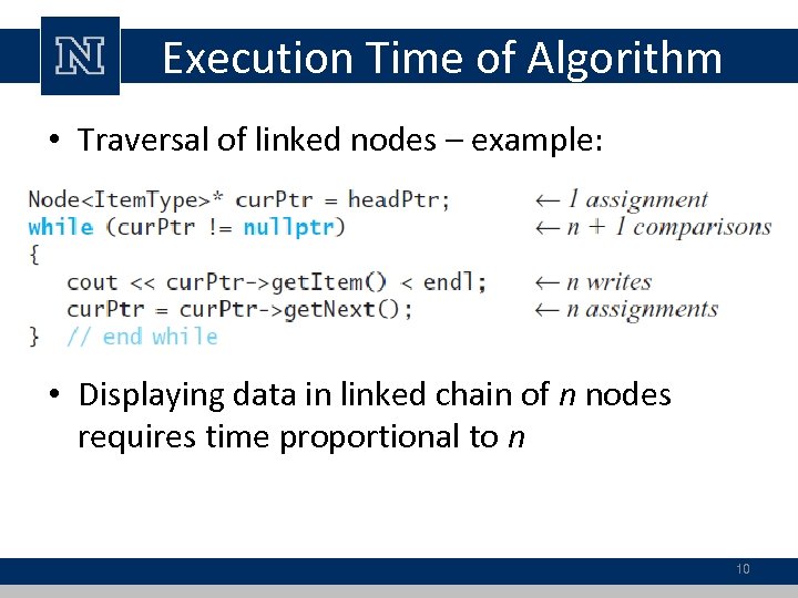Execution Time of Algorithm • Traversal of linked nodes – example: • Displaying data in linked chain of n nodes requires time proportional to n 10

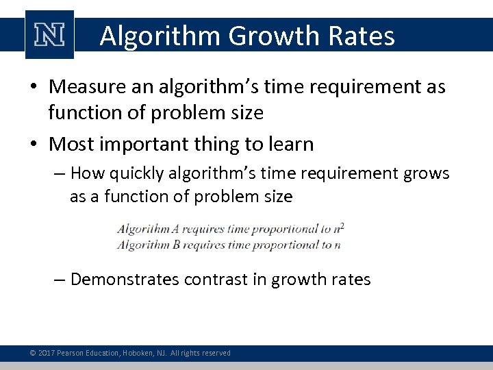Algorithm Growth Rates • Measure an algorithm’s time requirement as function of problem size • Most important thing to learn – How quickly algorithm’s time requirement grows as a function of problem size – Demonstrates contrast in growth rates © 2017 Pearson Education, Hoboken, NJ. All rights reserved

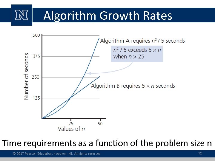Algorithm Growth Rates Time requirements as a function of the problem size n © 2017 Pearson Education, Hoboken, NJ. All rights reserved 12

Best, Worst, Average Cases • Not all inputs of a given size take the same time to run. • Sequential search for K in an array of n integers: – Begin at first element in array and look at each element in turn until K is found – Best case: – Worst case: – Average case: 13

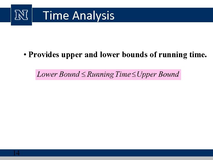Time Analysis • Provides upper and lower bounds of running time. 14

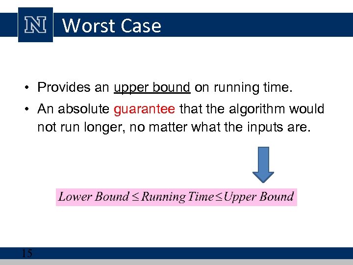Worst Case • Provides an upper bound on running time. • An absolute guarantee that the algorithm would not run longer, no matter what the inputs are. 15

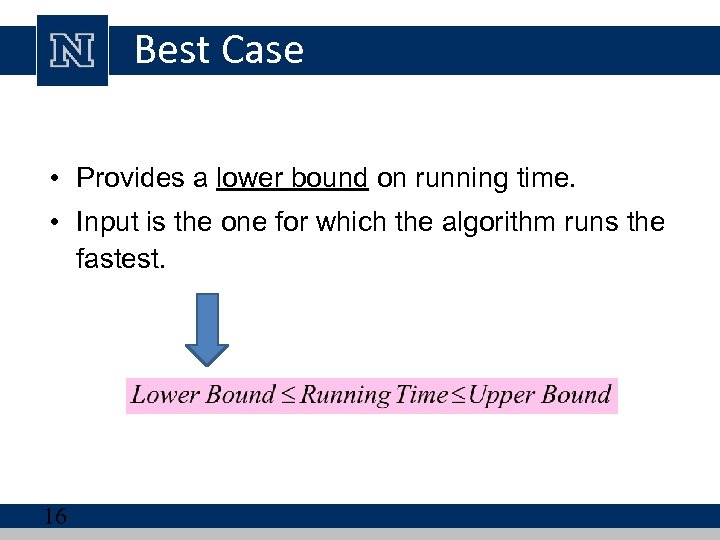Best Case • Provides a lower bound on running time. • Input is the one for which the algorithm runs the fastest. 16

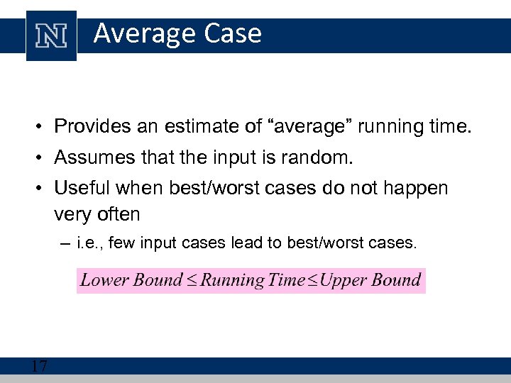Average Case • Provides an estimate of “average” running time. • Assumes that the input is random. • Useful when best/worst cases do not happen very often – i. e. , few input cases lead to best/worst cases. 17

Which Analysis to Use? • While average time appears to be the fairest measure, – it may be difficult to determine. • When is the worst case time important? 18

How to Measure Efficiency? • Critical resources: – Time, memory, battery, bandwidth, programmer effort, user effort • Factors affecting running time: – For most algorithms, running time depends on “size” of the input. – Running time is expressed as T(n) for some function T on input size n. 19

How do we analyze an algorithm? • Need to define objective measures. (1) Compare execution times? Empirical comparison (run programs) Not good: times are specific to a particular machine. (2) Count the number of statements? Not good: number of statements varies with programming language and programming style. 21

How do we analyze an algorithm? (cont. ) (3) Express running time t as a function of problem size n (i. e. , t=f(n) ) Asymptotic Algorithm Analysis - Given two algorithms having running times f(n) and g(n), - find which functions grows faster - Such an analysis is independent of machine time, programming style, etc. 22

Comparing algorithms • Given two algorithms having running times f(n) and g(n), how do we decide which one is faster? • Compare “rates of growth” of f(n) and g(n) 23

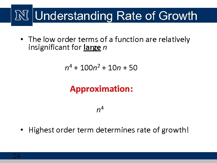Understanding Rate of Growth • The low order terms of a function are relatively insignificant for large n n 4 + 100 n 2 + 10 n + 50 Approximation: n 4 • Highest order term determines rate of growth! 24

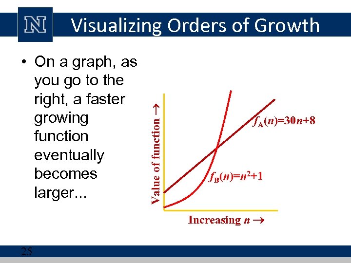• On a graph, as you go to the right, a faster growing function eventually becomes larger. . . Value of function Visualizing Orders of Growth f. A(n)=30 n+8 f. B(n)=n 2+1 Increasing n 25

Analysis and Big O Notation • Algorithm A is said to be order f (n), – Denoted as O( f (n)) – Function f(n) called algorithm’s growth rate function – Notation with capital O denotes order • Algorithm A of order denoted O(f(n)) – Constants k and n 0 exist such that – A requires no more than k f(n) time units – For problem of size n n 0 © 2017 Pearson Education, Hoboken, NJ. All rights reserved

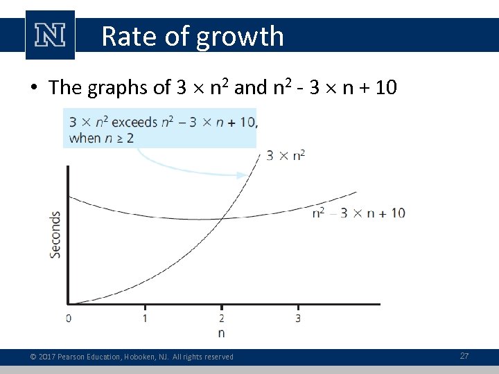Rate of growth • The graphs of 3 n 2 and n 2 - 3 n + 10 © 2017 Pearson Education, Hoboken, NJ. All rights reserved 27

Rate of Growth ≡ Asymptotic Analysis • Using rate of growth as a measure to compare different functions implies comparing them asymptotically – i. e. , as n • If f(x) is faster growing than g(x), then f(x) always eventually becomes larger than g(x) in the limit – i. e. , for large enough values of x 28

Complexity • Let us assume two algorithms A and B that solve the same class of problems. • The time complexity of A is 5, 000 n, the one for B is 1. 1 n for an input with n elements • For n = 10, – A requires 50, 000 steps, – but B only 3, – so B seems to be superior to A. • For n = 1000, A requires 5 106 steps, – while B requires 2. 5 1041 steps. 29

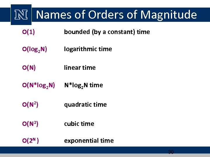Names of Orders of Magnitude O(1) bounded (by a constant) time O(log 2 N) logarithmic time O(N) linear time O(N*log 2 N) N*log 2 N time O(N 2) quadratic time cubic time O(N 3) O(2 N ) exponential time 30

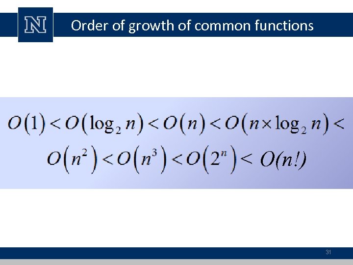Order of growth of common functions < O(n!) 31

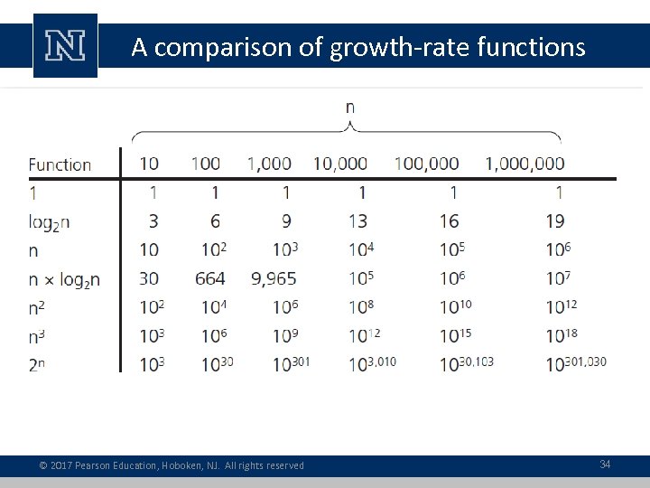
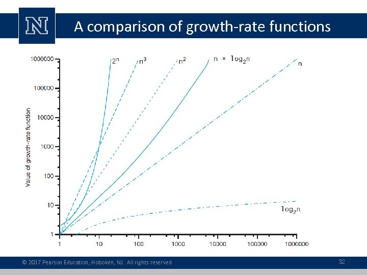A comparison of growth-rate functions © 2017 Pearson Education, Hoboken, NJ. All rights reserved 32

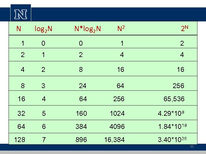N log 2 N N*log 2 N N 2 2 N 1 0 0 1 2 2 1 2 4 4 4 2 8 16 8 3 24 64 256 16 4 64 256 65, 536 32 5 160 1024 64 6 384 4096 128 7 896 16, 384 4. 29*109 1. 84*1019 3. 40*1038 33

A comparison of growth-rate functions © 2017 Pearson Education, Hoboken, NJ. All rights reserved 34

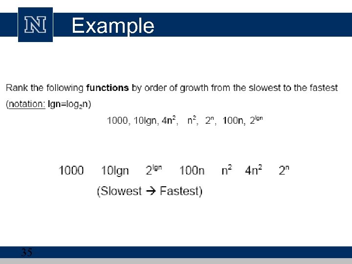Example 35

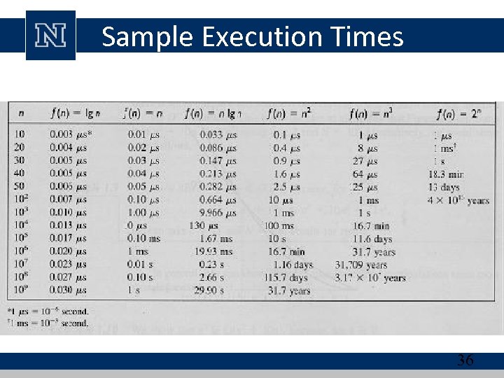Sample Execution Times 36

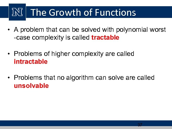The Growth of Functions • A problem that can be solved with polynomial worst -case complexity is called tractable • Problems of higher complexity are called intractable • Problems that no algorithm can solve are called unsolvable 37

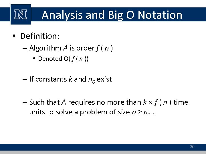Analysis and Big O Notation • Definition: – Algorithm A is order f ( n ) • Denoted O( f ( n )) – If constants k and n 0 exist – Such that A requires no more than k f ( n ) time units to solve a problem of size n ≥ n 0. 38

Analysis and Big O Notation • Worst-case analysis – Worst case analysis usually considered – Easier to calculate, thus more common • Average-case analysis – More difficult to perform – Must determine relative probabilities of encountering problems of given size © 2017 Pearson Education, Hoboken, NJ. All rights reserved

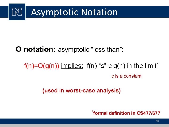Asymptotic Notation O notation: asymptotic “less than”: notation: f(n)=O(g(n)) implies: f(n) “≤” c g(n) in the limit* c is a constant (used in worst-case analysis) *formal definition in CS 477/677 40

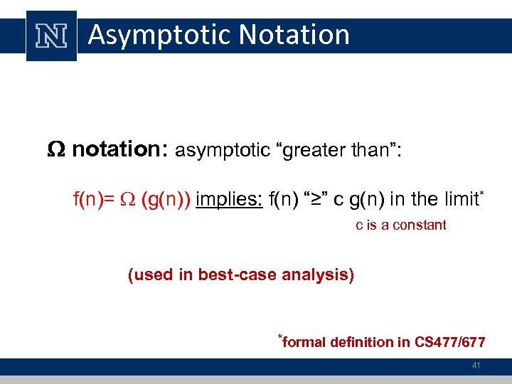Asymptotic Notation notation: asymptotic “greater than”: notation: f(n)= (g(n)) implies: f(n) “≥” c g(n) in the limit* c is a constant (used in best-case analysis) *formal definition in CS 477/677 41

Asymptotic Notation notation: asymptotic “equality”: notation: f(n)= (g(n)) implies: f(n) “=” c g(n) in the limit* c is a constant (provides a tight bound of running time) (best and worst cases are same) *formal definition in CS 477/677 42

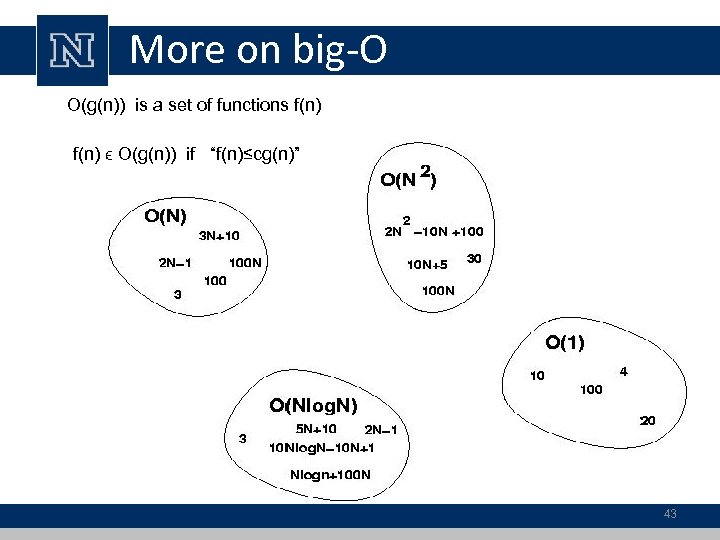More on big-O O(g(n)) is a set of functions f(n) ϵ O(g(n)) if “f(n)≤cg(n)” 43

A Common Misunderstanding • Confusing worst case with upper bound • Upper bound refers to a growth rate • Worst case refers to the worst input from among the choices for possible inputs of a given size 44

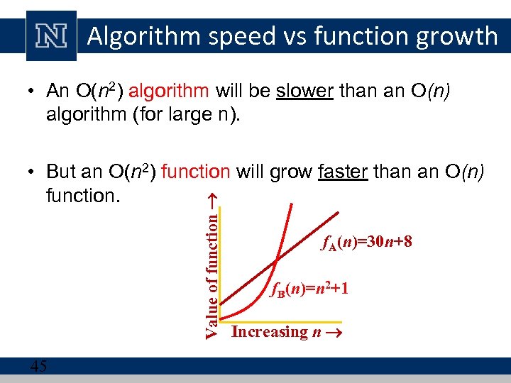Algorithm speed vs function growth • An O(n 2) algorithm will be slower than an O(n) algorithm (for large n). Value of function • But an O(n 2) function will grow faster than an O(n) function. 45 f. A(n)=30 n+8 f. B(n)=n 2+1 Increasing n

Keeping Your Perspective • Choosing implementation of ADT – Consider how frequently certain operations will occur – Seldom used but critical operations must also be efficient • If problem size is always small – Possible to ignore algorithm’s efficiency • Weigh trade-offs between – Algorithm’s time and memory requirements • Compare algorithms for style and efficiency © 2017 Pearson Education, Hoboken, NJ. All rights reserved

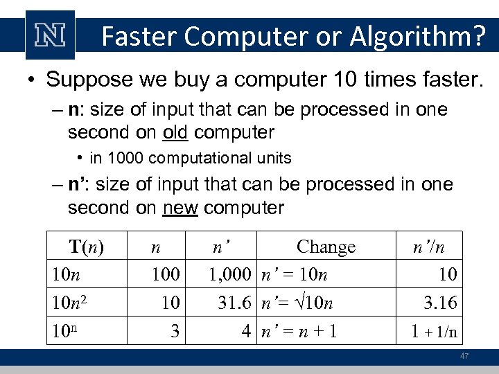Faster Computer or Algorithm? • Suppose we buy a computer 10 times faster. – n: size of input that can be processed in one second on old computer • in 1000 computational units – n’: size of input that can be processed in one second on new computer T(n) 10 n 2 10 n n 100 10 3 n’ Change 1, 000 n’ = 10 n 31. 6 n’= 10 n 4 n’ = n + 1 n’/n 10 3. 16 1 + 1/n 47

How do we find f(n)? (1) Associate a "cost" with each statement (2) Find total number of times each statement is executed (3) Add up the costs 48

Properties of Growth-Rate Functions • Ignore low-order terms • Ignore a multiplicative constant in the highorder term • O(f(n)) + O(g(n)) = O(f(n) + g(n)) • Be aware of worst case, average case 49

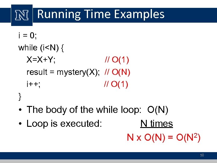Running Time Examples i = 0; while (i

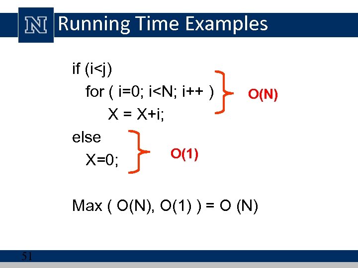Running Time Examples if (i

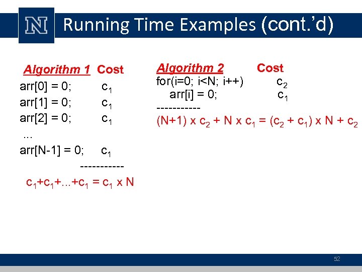Running Time Examples (cont. ’d) Algorithm 2 Cost Algorithm 1 Cost for(i=0; i

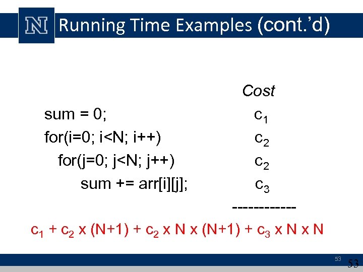Running Time Examples (cont. ’d) Cost sum = 0; c 1 for(i=0; i

Complexity Examples What does the following algorithm compute? int who_knows(int a[n]) { int m = 0; for {int i = 0; i m ) m = abs(a[i] – a[j]); return m; } returns the maximum difference between any two numbers in the input array Comparisons: n-1 + n-2 + n-3 + … + 1 = (n-1)n/2 = 0. 5 n 2 - 0. 5 n Time complexity is O(n 2) 54

Complexity Examples Another algorithm solving the same problem: int max_diff(int a[n]) { int min = a[0]; int max = a[0]; for {int i = 1; i max ) max = a[i]; return max-min; } Comparisons: 2 n - 2 Time complexity is O(n) 55

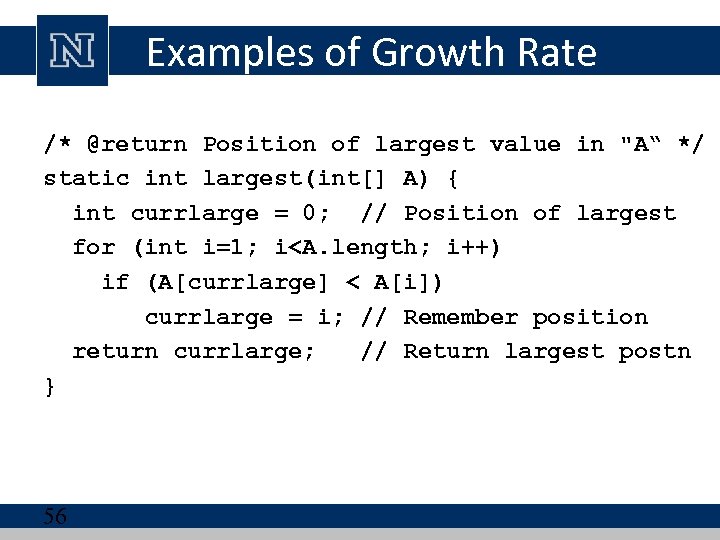Examples of Growth Rate /* @return Position of largest value in "A“ */ static int largest(int[] A) { int currlarge = 0; // Position of largest for (int i=1; i

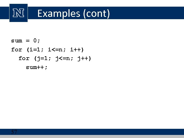Examples (cont) sum = 0; for (i=1; i<=n; i++) for (j=1; j<=n; j++) sum++; 57

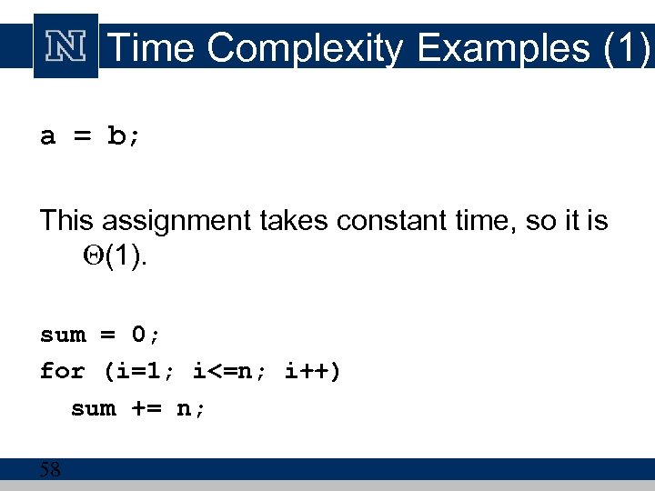Time Complexity Examples (1) a = b; This assignment takes constant time, so it is (1). sum = 0; for (i=1; i<=n; i++) sum += n; 58

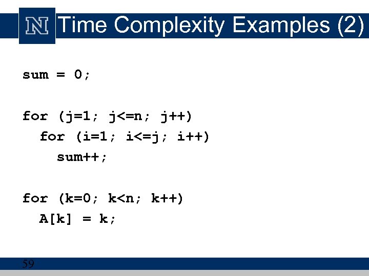Time Complexity Examples (2) sum = 0; for (j=1; j<=n; j++) for (i=1; i<=j; i++) sum++; for (k=0; k

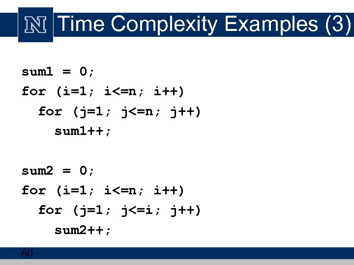Time Complexity Examples (3) sum 1 = 0; for (i=1; i<=n; i++) for (j=1; j<=n; j++) sum 1++; sum 2 = 0; for (i=1; i<=n; i++) for (j=1; j<=i; j++) sum 2++; 60

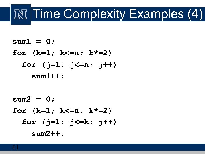Time Complexity Examples (4) sum 1 = 0; for (k=1; k<=n; k*=2) for (j=1; j<=n; j++) sum 1++; sum 2 = 0; for (k=1; k<=n; k*=2) for (j=1; j<=k; j++) sum 2++; 61

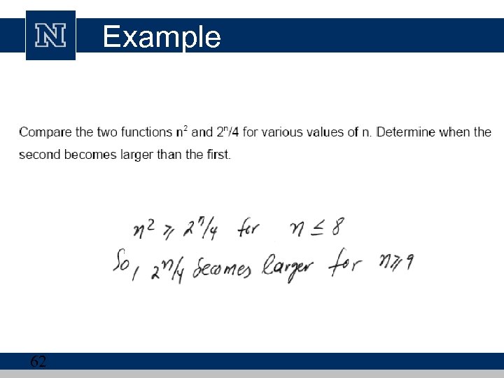Example 62

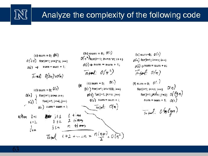Analyze the complexity of the following code 63