CHAPTER 1 CS 10051 TEXT READING ASSIGNMENT

CHAPTER 1 CS 10051

TEXT READING ASSIGNMENT Prefaces and Chapters 1 -2 OVERVIEW OF COURSE: 1. The algorithmic foundations of computer science. 2. The hardware world. 3. The virtual machine. 4. The software world. 5. Applications. 6. Social issues. Note these correspond to the labels on the step pyramid on the backside of first interior page of your text.

WHAT IS COMPUTER SCIENCE? MISCONCEPTION 1: Computer science is the study of computers. MISCONCEPTION 2: Computer science is the study of how to write computer programs. MISCONCEPTION 3: Computer science is the study of the uses and applications of computers and software.

SO, HOW DO WE DEFINE COMPUTER SCIENCE? Ø Computer science is the study of algorithms including l l 1. Their formal and mathematical properties 2. Their hardware realizations 3. Their linguistic realizations 4. Their applications

THAT LEADS TO THE OBVIOUS QUESTION: What is an algorithm? Ø An algorithm is a Ø well-ordered collection of Ø unambiguous and Ø effectively computable operations that, when executed, Ø produces a result and Ø halts in a finite amount of time.

AN EXAMPLE OF A VERY SIMPLE ALGORITHM Ø 1. Wet your hair. Ø 2. Lather your hair. Ø 3. Rinse your hair. Ø 4. Stop. Observe: Operations need not be executed by a computer only by an entity capable of carrying out the operations listed. We assume that The algorithm begins executing at the top of the list of operations. The "Stop" can be omitted if we assume the last line is an implied "Stop" operation.

A well-ordered collection of operations The question that must be answered is: At any point in the execution of the algorithm, do you know what operation is to be performed next? Well-ordered operations: Not well-ordered operations: 1. Wet your hair. 1. Either wet your hair or lather your hair. 2. Lather your hair. 3. Rinse your hair. 2. Rinse your hair.

Don't assume that you can't make choices: Well-ordered operations: 1. If your hair is dirty, then a. Wet your hair. b. Lather your hair. c. Rinse your hair. 2. Else a. Go to bed. Note: We will often omit the numbers and the letters and assume a "top-down" reading of the operations.

Unambiguous operations The question that must be answered is: Does the computing entity understand what the operation is to do? This implies that the knowledge of the computing entity must be considered. For example, is the following ambiguous? Make the pie crusts.

To an experienced cook, Make the pie crusts. is not ambiguous. But, an less experienced cook may need: Take 1 1/3 cups of flour. Sift the flour. Mix the sifted flour with 1/2 cup of butter and 1/4 cup of water to make dough. Roll the dough into two 9 -inch pie crusts. or even more detail!

Definition: An operation that is unambiguous is called a primitive operation (or just a primitive) One question we will be exploring in the course is what are the primitives of a computer. Note that a given collection of operations may be an algorithm with respect to one computing agent, but not with respect to another computing agent!!

Effectively computable operations The question that must be answered is: Is the computing entity capable of doing the operation? This assumes that the operation must first be unambiguous- i. e. the computing agent understands what is to be done. Not effectively computable operations: Write all the fractions between 0 and 1. Add 1 to the current value of x.

that, when executed, produces a result The question that must be answered is: Can the user of the algorithm observe a result produced by the algorithm? The result need not be a number or piece of text viewed as "an answer". It could be an alarm, signaling something is wrong. It could be an approximation to an answer. It could be an error message.

halts in a finite amount of time The question that must be answered is: Will the computing entity complete the operations in a finite number of steps and stop? Do not confuse "not finite" with "very, very large". A failure to halt usually implies there is an infinite loop in the collection of operations: 1. Write the number 1 on a piece of paper. 2. Add 1 to the number you just wrote and write it on a piece of paper. 3. Repeat 2. 4. Stop.

Definition of an algorithm: Ø An algorithm is a well-ordered collection of unambiguous and effectively computable operations that, when executed, produces a result and halts in a finite amount of time. Note: Although I have tried to give clean cut examples to illustrate what these new words mean, in some cases, a collection of operations can fail for more than one reason.

RETURNING TO OUR ORGINAL QUESTION: HOW DO WE DEFINE COMPUTER SCIENCE? Ø Computer science is the study of algorithms including l l 1. Their formal and mathematical properties 2. Their hardware realizations 3. Their linguistic realizations 4. Their applications

1. Their formal and mathematical properties Ø It is not enough to develop any old algorithm to solve a problem. Ø We must worry about some additional properties of an algorithm: l l l How efficient is it? What kinds of resources must be used to execute it? How does it compare to other algorithms that solve the same problem.

2. Their hardware realizations Ø Algorithms need not execute on machines. All we really need are computing entities. l Anything that can compute – e. g. , a human. Ø But, ultimately, most of our interest will lie with algorithms that execute on computing entities called "computers". Ø How are these entities constructed? l The emphasis will be on the logical construction of a computer, not the physical construction.

3. Their linguistic realizations Ø How do we represent algorithms? Ø We will start with one linguistic realization today, called pseudocode and later will look at many different realizations in various programming languages. Ø We'll even consider some of the visual representations using graphics.

And finally: 4. Their applications Ø What are some of the many important and popular applications of computers in current use including: l l l l modeling and simulation information retrieval numerical problem solving telecommunications artificial intelligence networking graphics

Early History of Computing Abacus An early device to record numeric values We normally do not call it a computer, but a computing device. It is still used in parts of the world today. This distinction between a computer and a computing device will become clearer as we look at other aspects of the history of computing. source: http: //www. ee. ryerson. ca: 8080/~elf/abacus/intro. html 6

Napier’s Bones (or Rods) Rods were marked with multiplication table results. Ø These were used to provide fairly simple means of multiplying large numbers. Ø On the below web site, one of the labs goes into some details on Napier’s Bones: http: //csilluminated. jbpub. com/labs/Napier. cfm Ø The honor for constructing the first calculating machine belongs to a German called Wilhelm Schickard. In 1623 he completed a mechanical calculating machine based on Napier's work. Ø

Using the bones to compute 46732 X 5 Add: 10 150 3500 30000 200000 source: http: //csilluminated. jbpub. com/labs/Napier. cfm

Slide Rule Ø Ø Ø In 1614, John Napier discovered algorithms which made it possible to perform multiplication and division using addition and subtraction. To avoid having to log tables, Edmund Gunter created a number line in which the position of numbers were proportional to their logs. William Oughtred soon simplified things further by creating a slide rule with two Gunter’s lines. l One line could “slide” in order to increment (multiply) or decrement (divide) a value by a second value. The slide rule was widely in use by the end of the 17 century and remained popular for the next 300 years. Improvements included ability to compute powers and roots of numbers but did not include ability to add or subtract.

Blaise Pascal In 1642 Blaise Pascal, a Frenchman invented a new kind of computing device. Ø It used wheels instead of beads. Each wheel had ten notches, numbered '0' to '9'. When a wheel was turned seven notches, it added 7 to the total on the machine. Ø Pascal's machine, known as the Pascaline, could add up to 999999. Ø It could also subtract. Ø source: http: //www. tased. edu. au/schools/rokebyh/curric/ infotech/stage 1/assign 2/pre 20 th. htm#schickard

Gottfried Leibnitz Ø Leibnitz improved on Pascal's adding machine so that it could also perform multiplication, division and calculate square roots. source: http: //www. tased. edu. au/schools/rokebyh/curric/ infotech/stage 1/assign 2/pre 20 th. htm#schickard

Grillet’s Pocket Calculator Ø Ø Ø One very early machine which incorporated Napier’s ideas was that built by a French clockmaker called Grillet in 1678. Grillet included a set of Napier's Rods in an adaptation of the Pascaline. It could be considered the world's first pocket calculator. The top section of the device consisted of 24 dials or sets of wheels. The lower section contained a set of inverted Napier’s Rods engraved on cylinders. Although the device was limited, it did allow simple operations to be performed. It could carry out eight digit additions -- something that would have been very useful at a time when very few people had skill with numbers.

Grillet’s Machine http: //www. tased. edu. au/schools/rokebyh/curric/infotech/stage 1/ assign 2/pre 20 th. htm#schickard

Joseph Jacquard In the late 1700 s in France, Joseph Jacquard invented a way to control the pattern on a weaving loom used to make fabric. Ø Jacquard punched pattern holes into paper cards. Ø The cards told the loom what to do. Ø Instead of a person making every change in a pattern, the machine made the changes all by itself. Ø Jacquard's machine didn't count anything. So it wasn't a computer or even a computing device. His ideas, however, led to many other computing inventions later. Ø

Jacquard Loom - A mechanical device that influenced early computer design Intricate textile patterns were prized in France in early 1800 s. Jacquard’s loom (1805 -6) used punched cards to allow only some rods to bring the thread into the loom on each shuttle pass. Source: http: //65. 107. 211. 206/technology/jacquard. html

Sheets of punched cards set the pattern of the weave Source: http: //65. 107. 211. 206/technology/jacquard. html

Luddites Ø Ø Ø Ø During the 1700's and early 1800's, part of the world saw the development of industrialization. Before the Industrial Revolution, manufacturing was done by hand or simple machines. The Industrial Revolution caused many people to lose their jobs. Groups of people known as Luddites attacked factories and wrecked machinery in Britain between 1811 and 1816. The Luddites received their name from their mythical leader Ned Ludd. They believed that the introduction of new textile machines in the early 1800's had caused unemployment and lowered the textile workers' standard of living. Note this is similar to the way some people see that computers today are taking the jobs of workers.

Charles Babbage is known as the father of modern computing because he was the first person to design a general purpose computing device. Ø In 1822, Babbage began to design and build a small working model of an automatic mechanical calculating machine, which he called a "difference engine". Ø Example: It could find the first In the Science Museum, 30 prime numbers in two and London a half minutes. Ø Source: http: //www. sciencemuseum. org. uk/online/babbage/page 3. asp

A closer look at difference engine source: http: //www. computer. org/history/development/graphics/diff_eng. jpg

Ø Babbage continued work to produce a full scale working Difference Engine for 10 years, but in 1833 he lost interest because he had a "better idea"--the construction of what today would be described as a general-purpose, fully program -controlled, automatic mechanical digital computer. Ø Babbage called his machine an "analytical engine". Ø He designed, but was unable to build, this Analytical Engine (1856) which had many of the characteristics of today’s computers: an input device – punched card reader an output device – a typewriter memory – rods which when rotated into position “stored” a number control unit – punched cards with instructions encoded as with the Jacquard loom

The machine was to operate automatically, by steam power, and would require only one attendant. source: http: //www. sciencemuseum. org. uk/on-line/babbage/page 5. asp

Some call Babbage’s analytic engine the first computer, but, as it was not built by him, most people place that honor elsewhere. Babbage's analytical engine contained all the basic elements of an automatic computer-storage, working memory, a system for moving between the two, an input device and an output device. Ø But Babbage lacked funding to build the machine so Babbage's computer was never completed. Ø

Babbage designed a printer, also, that has just been built at the Science Museum in London 4, 000 working parts! source: http: //news. bbc. co. uk/1/hi/sci/tech/710950. stm

Ada Lovelace Ada Byron Lovelace was a close friend of Babbage. Ø Ada thought so much of Babbage's analytical engine that she translated a previous work about the engine. Ø Because of the detailed explanations she added to the work, she has been called the inventor of computer programming. Ø Today, on behalf of her work in computing, a programming language, Ada, is named after her. source: http: //www. pbs. org/teachersource/mathline/concepts/ womeninmath/activity 2. shtm 7

Herman Hollerith Ø Ø Ø In 1886, Herman Hollerith invented a machine known as the Automatic Tabulating Machine, to count how many people lived in the United States. This machine was needed because the census was taking far too long. His idea was based on Jacquard's loom. Hollerith used holes punched in cards. The holes stood for facts about a person; such as age, address, or his type of work. The cards could hold up to 240 pieces of information. Hollerith also invented a machine, a tabulator, to select special cards from the millions. To find out how many people lived in Pennsylvania, the machine would select only the cards punched with a Pennsylvania hole. Hollerith's punched cards made it possible to count and keep records on over 60 million people.

Hollerith Tabulator Hollerith founded the Tabulating Machine Company. In 1924, the name of the company was changed to International Business Machines Corporation (IBM). This is the 1890 version used in tabulating the 1890 federal census. Source: http: //www. columbia. edu/acis/history/hollerith. html

Punched cards The punched card used by the Hollerith Tabulator for the 1890 US census. The punched card was standardized in 1928: It was the primary input media of data processing and computing from 1928 until the mid-1970 s and was still in use in voting machines in the 2000 USA presidential election. source: http: //www. columbia. edu/acis/history/hollerith. html

History of Hardware

Harvard Mark I, ENIAC, UNIVAC I, ABC and others These are the names of some of the early computers that launched a new era in mathematics, physics, engineering and economics initially and, subsequently, almost every area has been impacted by computers. Ø The early computers were huge physically and very limited by today’s standards. Ø

First Generation Hardware (1951 -1959) – Major characteristics Vacuum Tubes Large, not very reliable, generated a lot of heat Magnetic Drum Storage Memory device that rotated under a read/write head Card Readers & Magnetic Tape Drives Development of these sequential auxiliary storage devices 8

ABC built by Professor John Atanasoff and a graduate student, Clifford Berry, at Iowa State University between 1939 and 1942. Special purpose computer and was not truly programmable. Ø The instructions to the machine were entered by buttons. Ø Input: Punched paper tape Ø Output: Punched cards Ø Source: www. cs. iastate. edu/jva/images/abc-1942. gif

Mark I designed by Howard Aiken and Grace Hopper at Harvard University in 1939 -1944. Contains more than 750, 000 components, is 50 feet long, 8 feet tall, and weighs approximately 5 tons Instructions were pre-punched on paper tape Input was by punched cards Output was displayed on an electric typewriter. Could carry out addition, subtraction, multiplication, division and reference to previous results. Still exists in the Computer Science Building at Harvard University and can be turned on and run! Source: http: //www. digidome. nl/howard_h__aiken. htm

Zuse’s Machines, Z 1 -Z 4 built by Konrad Zuse in Berlin, Germany, 1938 – 1944 (all destroyed supposedly in the Berlin bombings) If these machines did exist as described by Zuse after the war, they were the first computers.

Rebuilt model of Z 3 housed in Deutsches Technik Museum, Berlin Input: from a numeric, decimal, 20 digit keyboard Output: Numbers displayed with lamps, 4 decimal digits with decimal point Programmed via a punch tape and punch tape reader Multiplication 3 seconds, division 3 seconds, addition 0. 7 seconds. Used a 600 relay numeric unit, 1600 relay storage unit

Computer vs computing device Ø Most, but not all, people claim a computer must be l l Digital Programmable Electronic General purpose Ø If any characteristic is missing, at best, you have a computing device.

Mauchly and Eckert or Zuse – built the first computer Many claim the ENIAC was the first computer as there was proof that it did exist. Ø John Mauchly envisioned the ENIAC. He was a professor of Physics at Ursinus College. In 1943 he attended a workshop at Penn were, he saw a machine calculating firing tables. Mauchly realized that he could build an electronic machine that could be much faster. Ø J. Presper Eckert solved the engineering challenges. The chief challenge was tube reliability. Eckert was able to get good reliability by running the tubes at 1/4 power. Ø

ENIAC – (Electrical Numerical Integrator And Calculator), built by Presper Eckert and John Mauchly at Moore School of Engineering, University of Pennsylvania, 1941 -46 Often called the first computer (that was electronic, programmable, general purpose and digital).

ENIAC 18, 000 vacuum tubes and weighed 30 tons Ø Duration of an average run without some failure was only a few hours, although it was predicted to not run at all! Ø When it ran, the lights in Philadelphia dimmed! Ø ENIAC Stored a maximum of twenty 10 -digit decimal numbers. Ø Input: IBM card reader Ø Output: Punched cards, lights Ø

Eniac’s Vacuum Tubes Photo taken at Computer Science History Museum, San Jose, CA, by Dr. Robert Walker on VLSI Trip to Silicon Valley.

A vacuum tube similar to those used in the earliest computers. Source: http: //www. cs. virginia. edu/brochure/images/mus_024. jpg

ENIAC Programming required rewiring of the machine, Source: http: //ftp. arl. army. mil/ftp/historic-computers/

UNIVAC – first commercial computer On March 31, 1951, the Census Bureau accepted delivery of the first UNIVAC computer. Ø The final cost was close to one million dollars. Ø Forty-six UNIVAC computers were built for both government and business uses. Ø Remington Rand became the first American manufacturer of a commercial computer system. Ø Their first non-government contract was for General Electric in Louisville, Kentucky, who used the UNIVAC computer for a payroll application. Ø source: http: //inventors. about. com/library/weekly/aa 062398. htm

UNIVAC’s prediction ignored A 1952 UNIVAC made history by predicting the election of Dwight D. Eisenhower as US president before the polls closed. Ø The results were not immediately reported by Walter Cronkite because they were not believed to be accurate. Ø Democratic presidential candidate Adlai Stevenson was the front-runner in all the advance opinion polls, but by 8: 30 p. m. on the East Coast, well before polls were closed in the Western states, UNIVAC projected 100 -to-1 odds that Dwight D. Eisenhower would win by a landslide, which is in fact what happened. Ø

1952 election night source: http: //www. cedmagic. com/history/univac-cronkite. html

Whirlwind at MIT - 1952 Ø The first digital computer capable of displaying real time text and graphics on a large oscilloscope screen. Bouncing ball displayed on screen Source: http: //www. accad. ohio-state. edu/~waynec/history/lesson 2. html

Second Generation Hardware (1959 -1965) - Characteristics Transistor Replaced vacuum tube, fast, small, durable, cheap Magnetic Cores Replaced magnetic drums, information available instantly Magnetic Disks Replaced magnetic tape, data can be accessed directly 9

A Typical Computing Environment in 1960 – UNIVAC 1107 at Case Institute of Technology source: http: //www. fourmilab. ch/documents/univac/case 1107. html

Ø 1961 - The true purpose of computers is finally realized in 1961, when a MIT student, Steve Russell, created the first computer game – Spacewar on a DEC PDP-1 - a minicomputer 200 hours to program! Sources: http: //inventors. about. com/library/weekly/aa 090198. htm http: //www. nersc. gov/~deboni/Computer. history/GAM. PDP-1/

Father of Graphics- Ivan Sutherland n. Ph. D. Thesis, 1963, MIT : n. Sketchpad: The First Interactive Computer Graphics Package on TX-2 (forerunner of DEC machines). Source: http: //www. sun. com/960710/feature 3/sketchpad. html#sketch

TX-2 was a giant machine for the day: 320 kilobytes of memory, about twice the capacity of the biggest commercial machines Ø magnetic tape storage, Ø an on-line typewriter, Ø the first Xerox printer, Ø paper tape for program input, Ø a light pen for drawing, Ø a nine inch CRT (i. e. display screen) ! Ø

Light Pen Input “Sketchpad: A Man-machine Graphical Communications System, " used the light pen to create engineering drawings directly on the CRT. Source: http: //www. accad. ohiostate. edu/~waynec/history/lesson 2. html

1964 CDC Control Data Corporation CDC 6600 at U of Texas, 1964 -68 Cost: $2, 000+ Kept in dustfree room behind locked doors source: http: //www. computerhistory. org/timeline. php? timeline_category=cmptr

CDC 6600 – University of Texas - 1964 Workstations were available to only a few. Most had to use punched cards handed in through a window Source: http: //ed-thelen. org/comp-hist/vs-cdc-6600. jpg

A sampling of 1960 -1965 circuit boards: Photo taken at Computer Science History Museum, San Jose, CA, by Dr. Robert Walker on VLSI Trip to Silicon Valley

Third Generation Hardware (19651971) Integrated Circuits Replaced circuit boards, smaller, cheaper, faster, more reliable. Transistors Now used for memory construction Terminal An input/output device with a keyboard and screen By 1968 you could buy a 1. 3 MHz CPU with half a megabyte of RAM and 100 megabyte hard drive for a mere US$1. 6 million. 10

PDP I – first of the minicomputers to be used by many universities.

The PDP-40, a popular 3 rd generation minicomputer in the early 1970’s

The DEC-10 was popular at a lot of large universities. Photo taken at Computer Science History Museum, San Jose, CA, by Dr. Robert Walker on VLSI Trip to Silicon Valley

Dumb terminals or workstations were used to tie into the mainframes: Photo taken at Computer Science History Museum, San Jose, CA, by Dr. Robert Walker on VLSI Trip to Silicon Valley

Fourth Generation Hardware (1971 -? ) Large-scale Integration Great advances in chip technology PCs, the Commercial Market, Workstations Personal Computers were developed as new companies like Apple and Atari came into being. Workstations emerged. 11

Personal Computers were Introduced around 1977

Photo of early PCs taken at Computer Science History Museum In San Jose, CA, by Dr. Robert Walker on Trip to Silicon Valley

Typical prices on early PCs Ø Contrary to Memory popular 16 K belief today, these were 32 K not cheap – the IBM 48 K 5100 in mid 1970 s. 64 K BASIC $8, 975 $11, 975 APL $9, 975 $12, 975 Both $10, 975 $13, 975 $14, 975 $15, 975 $16, 975 $17, 975 $18, 975 $19, 975 Note that $1 in 1975 would be equal to $3. 76 today so multiply these by ~3. 8! For this price comparison see http: //www. westegg. com/inflation/

VAX 780 – Early Math-CS computer at KSU, obtained in 1982.

Photo taken at Computer Science History Museum, San Jose, CA, by Dr. Robert Walker on VLSI Trip to Silicon Valley

Dumb terminals were used for some input with these machines and line printers were used for output: Photo taken at Computer Science History Museum, San Jose, CA, by Dr. Robert Walker on VLSI Trip to Silicon Valley

Parallel Computing and Networking Parallel Computing Computers rely on interconnected central processing units that increase processing speed. Networking With the Ethernet small computers could be connected and share resources. File servers connected PCs in the late 1980 s. ARPANET and LANs Internet 12

There are many different kinds of parallel machines – this is one type A parallel computer must be capable of working on one task even though many individual computers are tied together. Ø Lucidor is a distributed memory computer (a cluster) from HP. It consists of 74 HP servers and 16 HP workstations. Peak: 7. 2 GFLOPs Ø GFLOP = one billion decimal number operations/ second source: http: //www. pdc. kth. se/compresc/machines/lucidor. html

Cray Machines Are Another Type of Parallel Machine –Cray 1 Photo taken at Computer Science History Museum, San Jose, CA, by Dr. Robert Walker on VLSI Trip to Silicon Valley

Cray 2 Photo taken at Computer Science History Museum, San Jose, CA, by Dr. Robert Walker on VLSI Trip to Silicon Valley

Another Earlier Parallel Computer at the University of Illinois was the Illiac IV Photo taken at Computer Science History Museum, San Jose, CA, by Dr. Robert Walker on VLSI Trip to Silicon Valley

Another View of the Illiac IV Photo taken at Computer Science History Museum, San Jose, CA, by Dr. Robert Walker on VLSI Trip to Silicon Valley

CM-2 Connection Machine Interesting fact: The lights are there only for show!

The IBM 360 (late ’ 60 s) console created “blinking lights” expectation Photo taken at Computer Science History Museum, San Jose, CA, by Dr. Robert Walker on VLSI Trip to Silicon Valley

A History of the Web - Let’s Be Precise Ø Late 1960 s – the ARPANET was conceived as a network of computers in which packets of information (i. e. data) could be transmitted between various computers via telephone lines or higher speed dedicated data lines. Ø ARPA was the Advanced Research Projects Agency. Ø This allowed remote logins to computers (using telnet), the ability to transfer files between computers (using ftp = file transfer protocol), and e-mail.

Many people now say it was designed for the military, but that was newspaper hype. Ø The purpose of the ARPANET was to allow the sharing of National Science Foundation (NSF) research project information between researchers. Ø In 1972, there were 29 nodes (i. e. computer sites that were interconnected). Ø CS program at KSU was earliest node in Ohio (~1982). Ø

The ARPANET Introduced the Internet Protocol To move data from computer A to computer B: Break the data up into packets of information. l Each packet carries the IP (Internet Protocol) address of computer B which consists of 4 numbers. l At each computer, the address is read and then the envelope is shipped along to another computer using a recipe called a routing algorithm. l At no time are A and B necessarily physically connected (unless they are adjacent nodes on the network). l The different packets will not necessarily follow the same route. l At computer B, the packets are reassembled into the document. l A packet is typically in the 40 – 1500 byte range (1 byte = 1 character) l

Document X at A Packet-based transmission of a document from Computer A to Computer B Note: If one computer fails, the document still may be transmitted. Packet X-1 for B Computer C Packet X-2 for B Computer F Packet X-3 for B Computer E Computer D Computer B Computer G Document X at B

Tracing the Route Your Packets Take Traceroute is a tool that traces the route your packets take. Ø Ping is a tool that tells you whether or not a web site is up. Ø Ping Plotter (http: //www. pingplotter. com/) is a tool that graphically shows you the route your packets take. l It was free, but can be used for 30 days without a subscription of $0. 99 a month today. l Interesting to see how your packets travel! Ø

One Ping Plotter Trace to www. weather. com

A Trace to KSU If you watch these interactively you’ll see the route changes.

Internet to World Wide Web The Internet is a collection of computers using the internet protocol to transmit information Ø The World Wide Web is a multimedia environment invented by Tim Berners-Lee, in 1990. l Was a physicist at CERN (the European Organization for Nuclear Research). l Wrote the first web browser (World. Wide. Web) and the software for the first web server. l Invented both the HTML markup language in which many web pages are written and the HTTP protocol used to request and transmit web pages between web servers and web browsers Ø

Growth in WWW Ø Number of Unique Web Sites The number of Web sites, adjusted to account for sites duplicated at multiple IP addresses. 1998: 2, 636, 000 1999: 4, 662, 000 2000: 7, 128, 000 2001: 8, 443, 000 2002: 8, 712, 000 Ø A Web site is defined as a distinct location on the Internet, identified by an IP address, that returns a response code of 200 and a Web page in response to an HTTP request for the root page. The Web site consists of all interlinked Web pages residing at the IP address. Ø Statistics provided by OCLC Online Computer Library Center, Inc. , Office of Research

Active Internet Users by Major Country

Average Web Usage in U. S.

More Than Half of People in U. S. and Canada Regularly Use Internet

Global Usage – Includes All Countries Monitored : ~20 countries accounting an estimated 90% of all Internet users For a more complete list see: http: //www. clickz. com/stats/big_picture/geographics/article. php/ 5911_151151

From the “Computer Industry Almanac” Ø Worldwide Internet Population 2004: 934 million Ø Projection for 2005: 1. 07 billion Ø Projection for 2006: 1. 21 billion Ø Projection for 2007: 1. 35 billion For more details for individual countries see: http: //www. clickz. com/stats/sectors/geographics/ article. php/%205911_151151

Negative Properties of WW Uneven capabilities of user’s browsers and other software l i. e. plug-ins differ widely and can interact with each other in strange ways. Ø No central control – therefore, unregulated and somewhat uncensored. Ø Anonymity of site owners. Ø Contrary to popular belief, it is not free. Ø Device independent – but not all hardware acts the same. Ø Copyright issues are more pronounced. Ø Uneven bandwidth – number of bits that can be transmitted per second. Ø

Be Cautious and Critical Ø There is a famous New Yorker cartoon: Cartoon by Peter Steiner reproduced from page 61 of July 5, 1993 issue of The New Yorker, (Vol. 69 (LXIX) no. 20).

Brief Mention of History of Theory We’ll study this more later

Alan Turing Machine, Artificial Intelligence Testing Ø Ø Ø Much of the early work on computers was theoretical and done by mathematicians. Alan Turing, and others, studied the questions “What tasks can be computed? ” and “What is a computer? ” His abstract model, called the Turing Machine, is of great interest in studying these questions. Another big questions was, and still is, “Are machines intelligent? ” Alan Turing devised a test, now known as The Turing Test (1950), to answer this question. We’ll delve into these issues a little later in the course.

History of Software Again, we will go deeper into these topics later

First Generation Software (1951 -1959) -we’ll see more on these topics later Machine Language Computer programs were written in binary (1 s and 0 s) Assembly Languages and translators Programs were written in languages that mimicked machine language and were then translated into machine language Programmers begin to specialize Programmers divide into application programmers and systems programmers. 13

Systems vs Applications Ø Computer scientists that design programs and systems for other computer scientists to use are called systems computer scientists. Ø Computer scientists that design programs and systems for non-computer scientists to use are called application computer scientists.

Second Generation Software (1959 -1965) High Level Languages Use English-like statements and made programming easier: Fortran, COBOL, Lisp. High-Level Languages Assembly Language Machine Language 14

Third Generation Software (19651971) Ø Systems Software Developed l l l utility programs, language translators, and the operating system, which decides which programs to run and when. Separation between Users and Hardware Ø Computer programmers now created programs to be used by people who did not know how to program Ø 15

Third Generation Software (19651971) Application Package Systems Software High-Level Languages Assembly Language Machine Language 16

Fourth Generation Software (19711989) Structured Programming Pascal, C New Application Software for Users Spreadsheets, word processors, database management systems 17

Fifth Generation Software (1990 present) Microsoft The Windows operating system, and other Microsoft application programs dominate the market Object-Oriented Design Based on a hierarchy of data objects (i. e. Java, C++) World Wide Web Allows easy global communication through the Internet New Users Today’s user can “get by” with little computer knowledge 18

Computing as a Tool Programmer / User Systems Programmer (builds tools) Applications Programmer (uses tools) Domain-Specific Programs User with No Computer Background 20

Computing as a Discipline Ø What can be (efficiently) Automated? Ø Four Necessary Skills 1. 2. 3. 4. Algorithmic Thinking Representation Programming Design 21

Some Systems Areas of Computer Science Ø Study of Algorithms and Data Structures Ø Programming Languages Ø Architecture Ø Operating Systems Ø Software Methodology and Engineering Ø Human-Computer Communication Ø Systems Programming 23

Some Application Areas of Computer Science Ø Numerical and Symbolic Computation Ø Databases and Information Retrieval Ø Artificial Intelligence and Robotics Ø Graphics Ø Organizational Informatics Ø Bioinformatics Ø Multimedia Ø Game development 24

Some other disciplines sharing some ground with computer science Ø Computer engineering Ø Electrical engineering Ø Computational physics Ø Computational chemistry Ø Computational biology (or bioinformatics)

Hot off the presses What field has… • …the best-rated job, and 5 of the top 10 highest paid, highest growth jobs? • …shown strong job growth in the face of outsourcing? • …a looming severe shortage in college graduates? Computer Science! This slide and the rest of the slides in this presentation were collated from SIGCSE announcements and displayed at the Gettysburg College Department of Computer Science website. Individual sources are given on the last slide.

Ø • Software engineers top the list of best jobs according to a Money magazine and Salary. com survey based on “strong growth prospects, average pay of $80, 500 and potential for creativity”. [1]

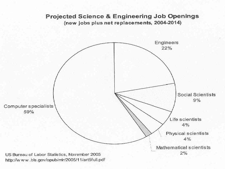
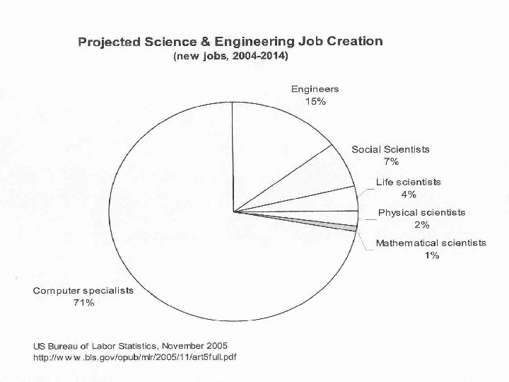
Ø 5 computing jobs are in the top 10 salary jobs from the Bureau of Labor Statistics’ list of the 30 fastest growing jobs through 2014. [2] 1. Computer systems software engineer: $81, 140 2. Computer applications software engineer: $76, 310 6. Computer systems analyst: $67, 520 7. Database administrator: $61, 950 9. Network systems and data communication analyst: $61, 250 Salaries are given as mean annual salaries over all regions.

• In April 2006, more Americans were employed in IT than at any time in the nation’s history. [3] • In May 2004, “U. S. IT employment was 17% higher than in 1999 5% higher than in 2000 and showing an 8% growth in the [following] year … The compound annual growth rate of IT wages has been about 4% since 1999 while inflation has been just 2% per year … Such growth rates swamp predictions of the outsourcing job loss in the U. S. , which most studies estimate to be 2% to 3% per year for the next decade. ” [4]

• “According to the National Science Foundation, the need for science and engineering graduates will grow 26%, or by 1. 25 million, between now and 2012. The number of jobs requiring technical training is growing at five times the rate of other occupations. And U. S. schools are nowhere near meeting the demand, according to multiple studies. ” [5] • The percentage of college freshmen listing computer science as their probable major fell 70% between 2000 and 2004. [6]

[1] Wulfhorst, Ellen. Reuters. com, Apr. 12, 2006. http: //www. salary. com/careers/layoutscripts/crel_display. asp? tab=cre&cat=nocat&ser=Ser 387&part=Par 615 [2] Morsch, Laura. Career. Builders. com, Jan. 27, 2006. http: //www. cnn. com/2006/US/Careers/01/26/cb. top. jobs. pay/index. html [3] Chabrow, Eric. Information. Week. com, Apr. 18, 2006. http: //www. informationweek. com/show. Article. jhtml? article. ID=185303797 [4] Patterson, David. President’s Letter: Restoring the Popularity of Computer Science, Communications of the ACM, Sept. 2005, Vol. 48, No. 9 [5] Deagon, Brian. Investor’s Business Daily, May 12, 2006. http: //www. investors. com/editorial/IBDArticles. asp? artsec=24&issue=20060512&view=1 [6] Robb, Drew. Computer. World. com, July 17, 2006. http: //computerworld. com/action/article. do? command=print. Article. Basic&article. Id=112364