Chapter 1 Choices 1 Definition of Game

Chapter 1 Choices 1

Definition of Game Theory • Game theory provides a framework in which to model and analyze conflict and cooperation among different entities, each with its own goal 2

Objective Function • When faced with a decision, we want the best choice for us. • Need to maximize an objective function (which measures our benefit from the decision) • Example: buying a house. Want more space or smaller house in better location • Example: budget – what activity gets what money 3

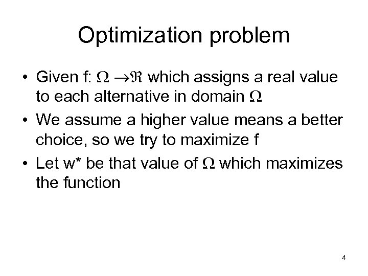Optimization problem • Given f: which assigns a real value to each alternative in domain • We assume a higher value means a better choice, so we try to maximize f • Let w* be that value of which maximizes the function 4

Example • Want to buy apples and oranges. Apples cost $1 per pound and oranges $2 per pound. • We have $12 total. • (x, y) represents buying x apples and y oranges. • Let f(x, y) = xy represent the worth of the choice (x, y). Which is better (12, 0), (6, 3), or (5, 1)? • We need to define the domain. is the set {(x, y) | x 0, y 0, x + 2 y 12} • How could you find the optimal solution? 5

Relative versus absolute extremum • • Extrema (c, d, e, f) Maxima (c, d) minima (e, f) Relative (c, e) vs. absolute (d, f) extrema Local (c, e) vs. global (d, f) extrema D y C E F x 6

Critical & stationary values • The critical value of x is the value x* if f ’(x*) = 0 • A stationary point is a point at which the derivative of a function f(x) vanishes • A stationary point may be a minimum, maximum, or inflection point. • A stationary value (The value at a stationary point) of y is f(x*) • A stationary point is the point with coordinates x* and f(x*) 7

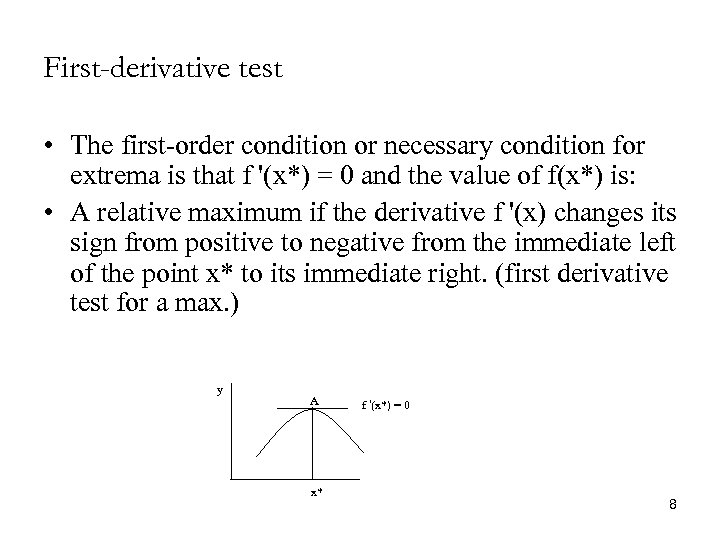First-derivative test • The first-order condition or necessary condition for extrema is that f '(x*) = 0 and the value of f(x*) is: • A relative maximum if the derivative f '(x) changes its sign from positive to negative from the immediate left of the point x* to its immediate right. (first derivative test for a max. ) y A x* f '(x*) = 0 8

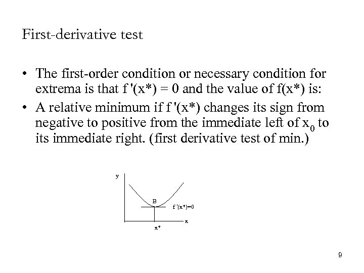First-derivative test • The first-order condition or necessary condition for extrema is that f '(x*) = 0 and the value of f(x*) is: • A relative minimum if f '(x*) changes its sign from negative to positive from the immediate left of x 0 to its immediate right. (first derivative test of min. ) y B x* f '(x*)=0 x 9

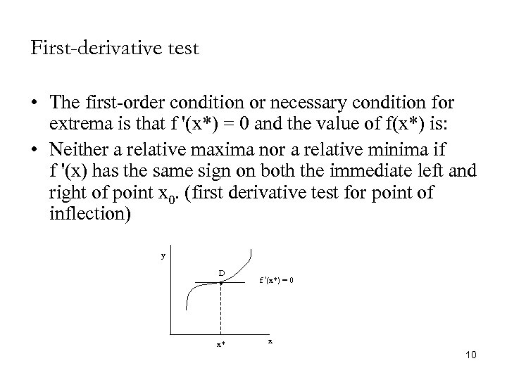First-derivative test • The first-order condition or necessary condition for extrema is that f '(x*) = 0 and the value of f(x*) is: • Neither a relative maxima nor a relative minima if f '(x) has the same sign on both the immediate left and right of point x 0. (first derivative test for point of inflection) y D x* f '(x*) = 0 x 10

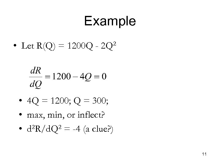Example • Let R(Q) = 1200 Q - 2 Q 2 • 4 Q = 1200; Q = 300; • max, min, or inflect? • d 2 R/d. Q 2 = -4 (a clue? ) 11

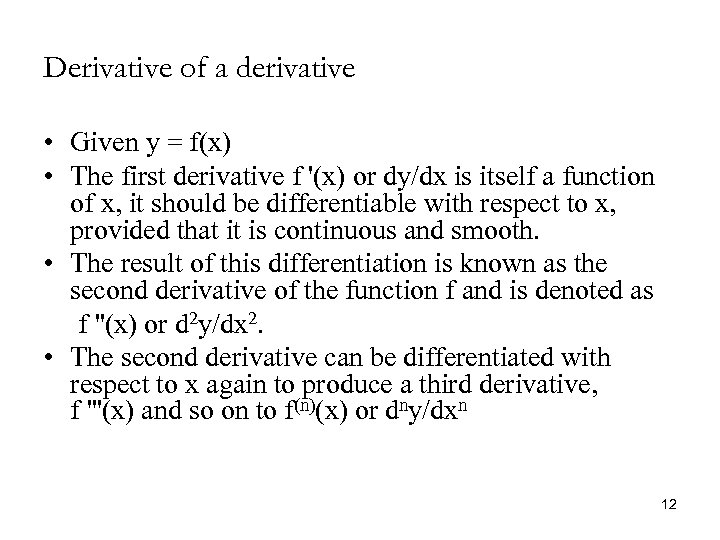Derivative of a derivative • Given y = f(x) • The first derivative f '(x) or dy/dx is itself a function of x, it should be differentiable with respect to x, provided that it is continuous and smooth. • The result of this differentiation is known as the second derivative of the function f and is denoted as f ''(x) or d 2 y/dx 2. • The second derivative can be differentiated with respect to x again to produce a third derivative, f '''(x) and so on to f(n)(x) or dny/dxn 12

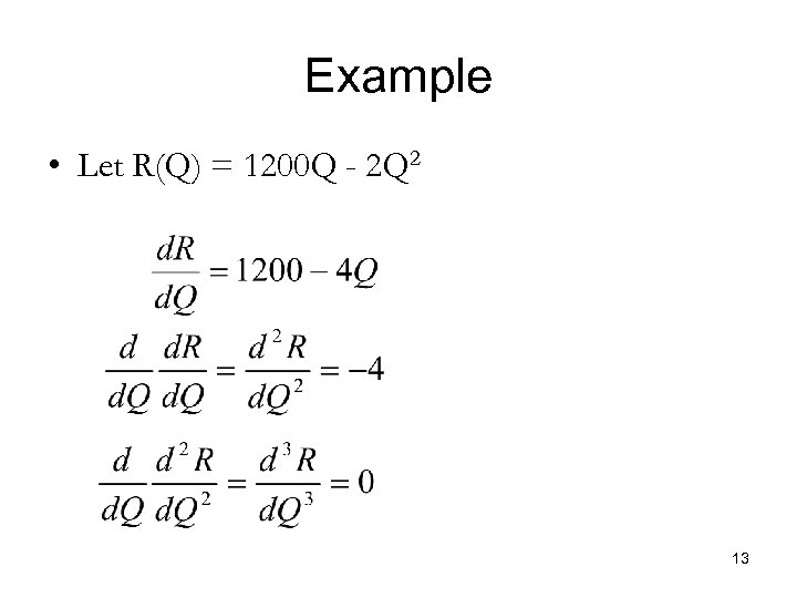Example • Let R(Q) = 1200 Q - 2 Q 2 13

Interpretation of the second derivative • f '(x) measures the rate of change of a function – e. g. , whether the slope is increasing or decreasing • f ''(x) measures the rate of change in the rate of change of a function – e. g. , whether the slope is increasing or decreasing at an increasing or decreasing rate 14

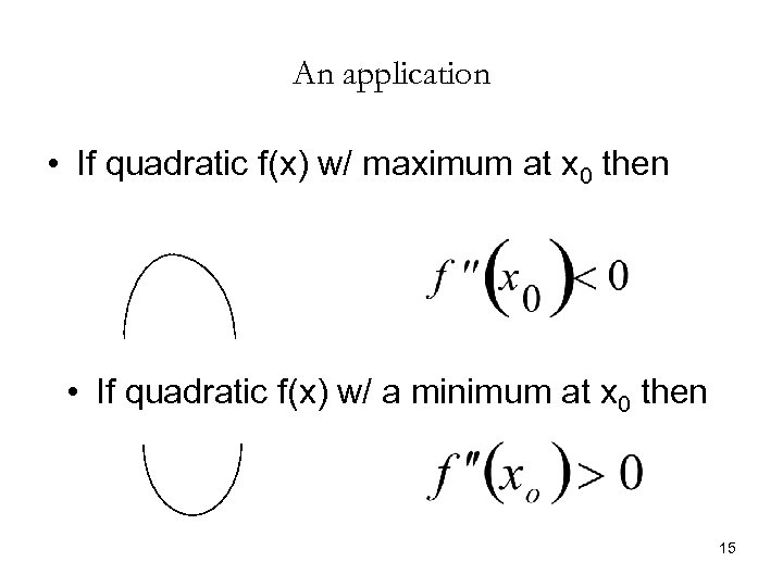An application • If quadratic f(x) w/ maximum at x 0 then • If quadratic f(x) w/ a minimum at x 0 then 15

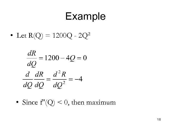Example • Let R(Q) = 1200 Q - 2 Q 2 • Since f''(Q) < 0, then maximum 16

• profit function (on left in red) with 1 st derivative shown in blue. • on right, 1 st deriviative is shown again (on different scale) and its deriviate (the 2 nd derivative) is shown in red, 17

Figure 1. 2 • Shows the set of possible choices for our problem of apples and oranges. • Does not show you how the maximum is found. y 6 utility maximizer: (6, 3) budget line: x+2 y=12 budget set x 12 18

How is maximum found? • • Have two functions u(x, y) = xy (utility function) x+2 y 12 u(y) = (12 -2 y)*y = 12 y-2 y 2 Need to maximize u u’(y) = 12 -4 y = 0 y=3 x=6 19

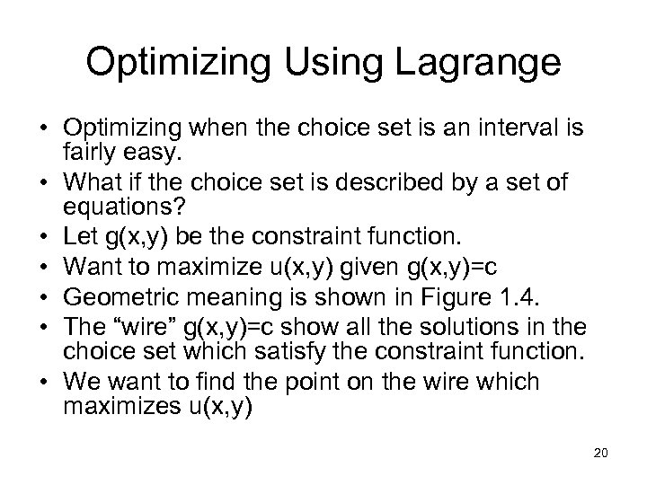Optimizing Using Lagrange • Optimizing when the choice set is an interval is fairly easy. • What if the choice set is described by a set of equations? • Let g(x, y) be the constraint function. • Want to maximize u(x, y) given g(x, y)=c • Geometric meaning is shown in Figure 1. 4. • The “wire” g(x, y)=c show all the solutions in the choice set which satisfy the constraint function. • We want to find the point on the wire which maximizes u(x, y) 20

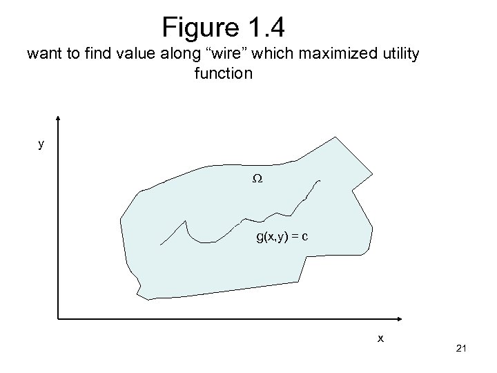Figure 1. 4 want to find value along “wire” which maximized utility function y g(x, y) = c x 21

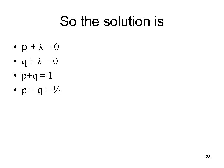
Lagrange Method • • Maximize u(x, y) under constraint g(x, y)=c Create the equation L(x, y, λ )= u(x, y) + λ(c-g(x, y)) Find maximums by setting all partial derivates (with respect to x, y and λ) to zero • For example, maximize pq under the constraint: p+q=1 • Lagrange Method: – Define L(p, q)=pq+λ(p+q-1) – Solve the equations 22

So the solution is • • p+λ=0 q+λ=0 p+q = 1 p=q=½ 23

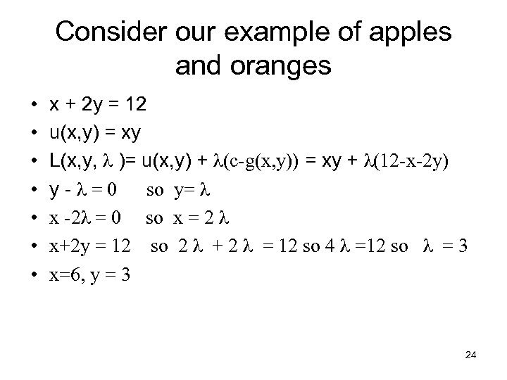Consider our example of apples and oranges • • x + 2 y = 12 u(x, y) = xy L(x, y, λ )= u(x, y) + λ(c-g(x, y)) = xy + λ(12 -x-2 y) y-λ=0 so y= λ x -2λ = 0 so x = 2 λ x+2 y = 12 so 2 λ + 2 λ = 12 so 4 λ =12 so λ = 3 x=6, y = 3 24

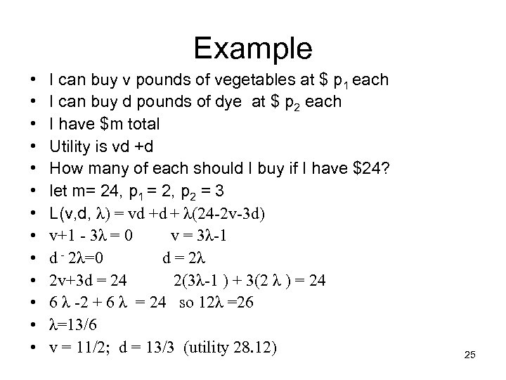Example • • • • I can buy v pounds of vegetables at $ p 1 each I can buy d pounds of dye at $ p 2 each I have $m total Utility is vd +d How many of each should I buy if I have $24? let m= 24, p 1 = 2, p 2 = 3 L(v, d, λ) = vd +d + λ(24 -2 v-3 d) v+1 - 3λ = 0 v = 3λ-1 d - 2λ=0 d = 2λ 2 v+3 d = 24 2(3λ-1 ) + 3(2 λ ) = 24 6 λ -2 + 6 λ = 24 so 12λ =26 λ=13/6 v = 11/2; d = 13/3 (utility 28. 12) 25

Example 1. 6 • Can manufacture x units of product at factory A costing 2 x 2 + 50000 • Can manufacture y units of product at factory B costing y 2 + 40000 • We want to minimize cost but need to produce 1200 units total. • L(x, y, λ) = 2 x 2 + 50000 + y 2 + 40000 + λ(1200 -x+y) • 4 x - λ = 0 2 y - λ = 0 x+y = 1200 • x = λ /4 y = λ /2 3λ /4 = 1200 • λ=1600 • x = 400, y = 800 26

Uncertainty and Chance • In decision making, often you don’t know what the other player will do, but only have some guesses of what he will do. • Thus, we need to deal with our estimates of what they will do - probability • A probability space (S, P) where S is a finite set, called the sample space, and P is a function that assigns a probability to elements si in S • pi 0 and pi = 1 where pi is the probabilty of si • if A is a subset of S then, P(A) = pi (when si A) 27

• subsets of the sample space are called events • Events are random outcomes of chance • Throwing coins has events H (throwing heads) and T (throwing tails) • P(H) = P(T) = ½ • A random variable, X, is a function from S to the Reals. It converts an event like “throw a head” to a number. Makes it easier to work with all events in a similar manner. • Say X(H) = 1 and X(T) = 2. 28

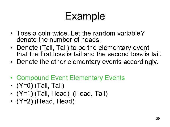Example • Toss a coin twice. Let the random variable. Y denote the number of heads. • Denote (Tail, Tail) to be the elementary event that the first toss is tail and the second toss is tail. • Denote the other elementary events accordingly. • • Compound Event Elementary Events (Y=0) (Tail, Tail) (Y=1) (Tail, Head), (Head, Tail) (Y=2) (Head, Head) 29

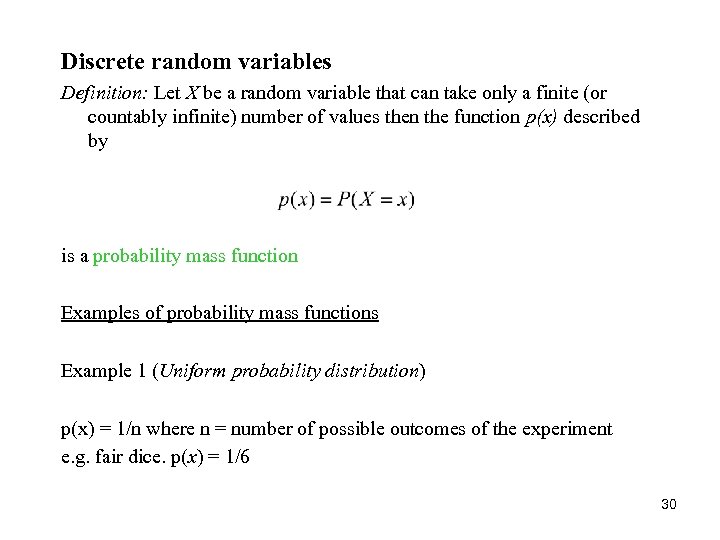Discrete random variables Definition: Let X be a random variable that can take only a finite (or countably infinite) number of values then the function p(x) described by is a probability mass function Examples of probability mass functions Example 1 (Uniform probability distribution) p(x) = 1/n where n = number of possible outcomes of the experiment e. g. fair dice. p(x) = 1/6 30

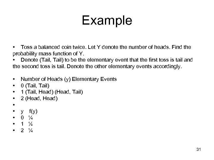Example • Toss a balanced coin twice. Let Y denote the number of heads. Find the probability mass function of Y. • Denote (Tail, Tail) to be the elementary event that the first toss is tail and the second toss is tail. Denote the other elementary events accordingly. • • • Number of Heads (y) Elementary Events 0 (Tail, Tail) 1 (Tail, Head) (Head, Tail) 2 (Head, Head) y f(y) 0 ¼ 1 ½ 2 ¼ 31

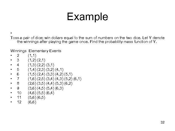Example • Toss a pair of dice; win dollars equal to the sum of numbers on the two dice. Let Y denote the winnings after playing the game once. Find the probability mass function of Y. Winnings • 2 • 3 • 4 • 5 • 6 • 7 • 8 • 9 • 10 • 11 • 12 Elementary Events (1, 1) (1, 2) (2, 1) (1, 3) (2, 2) (3, 1) (1, 4) (2, 3) (3, 2) (4, 1) (1, 5) (2, 4) (3, 3) (4, 2) (5, 1) (1, 6) (2, 5) (3, 4) (4, 3) (5, 2) (6, 1) (2, 6) (3, 5) (4, 4) (5, 3) (6, 2) (3, 6) (4, 5) (5, 4) (6, 3) (4, 6) (5, 5) (6, 4) (5, 6) (6, 5) (6, 6) 32

Properties of Probability Mass Functions (Discrete probability distributions) for all x p(x) = 1 Definition: Distribution Function The term distribution function is short for cumulative distribution function and describes the integral of the probability density function Let X be a random variable. Then F(x) = is called the distribution function of X. A discrete random variable can be represented as a histogram. For a discrete random variable, F(x) is just the sum of the area of the boxes of a histogram below and including x. 33

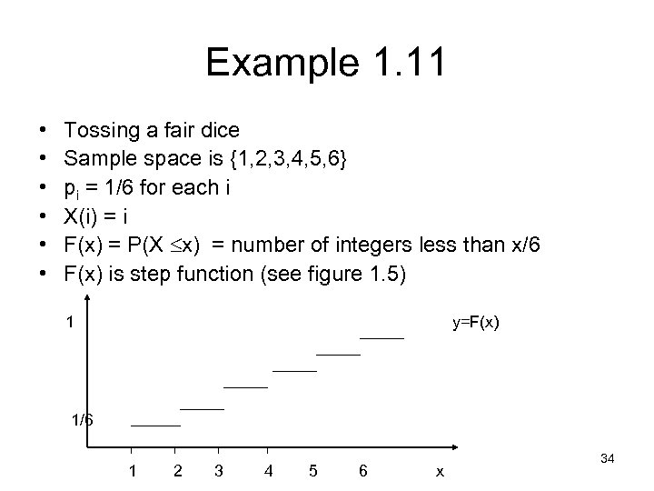Example 1. 11 • • • Tossing a fair dice Sample space is {1, 2, 3, 4, 5, 6} pi = 1/6 for each i X(i) = i F(x) = P(X x) = number of integers less than x/6 F(x) is step function (see figure 1. 5) 1 y=F(x) 1/6 1 2 3 4 5 6 x 34

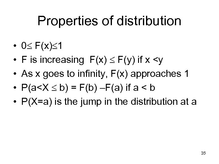Properties of distribution • • • 0 F(x) 1 F is increasing F(x) F(y) if x

Uniform Distribution • X has a uniform distribution on interval [a, b] if f(x) = 1/(b-a) if a

Normal Distribution • Bell-shaped, symmetric family of distributions • Classified by 2 parameters: Mean (m) and standard deviation (s). These represent location and spread • Random variables that are approximately normal have the following properties with respect to individual measurements: – Approximately half (50%) fall above (and below) mean – Approximately 68% fall within 1 standard deviation of mean – Approximately 95% within 2 standard deviations of mean – Virtually all fall within 3 standard deviations of mean • Notation when Y is normally distributed with mean m and standard deviation s : 37

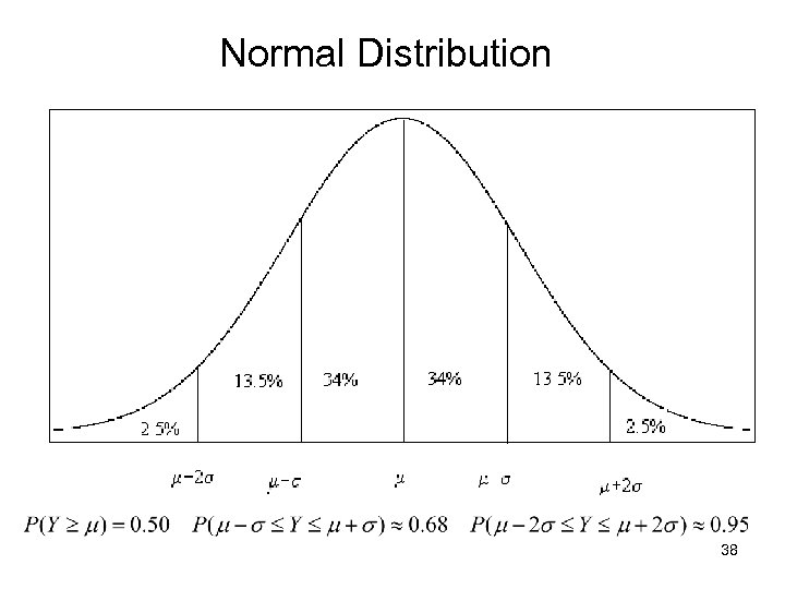Normal Distribution 38

Example - Heights of U. S. Adults • Female and Male adult heights are well approximated by normal distributions: YF~N(63. 7, 2. 5) YM~N(69. 1, 2. 6) 39 Source: Statistical Abstract of the U. S. (1992)

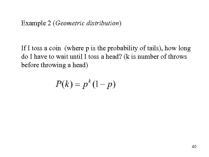Example 2 (Geometric distribution) If I toss a coin (where p is the probability of tails), how long do I have to wait until I toss a head? (k is number of throws before throwing a head) 40

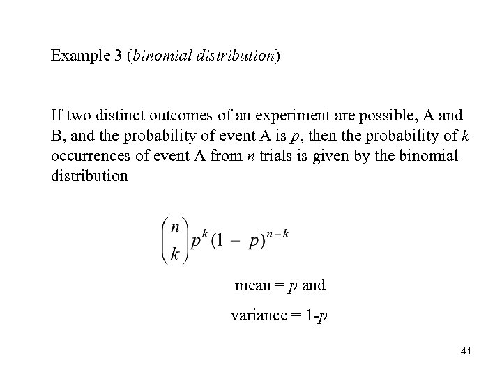Example 3 (binomial distribution) If two distinct outcomes of an experiment are possible, A and B, and the probability of event A is p, then the probability of k occurrences of event A from n trials is given by the binomial distribution mean = p and variance = 1 -p 41

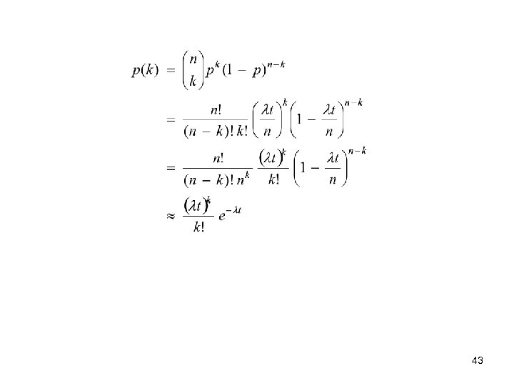
Example 5 (Poisson distribution) Poisson distribution: Discrete probability distribution for context-independent ‘rare’ events Say events occur at some rate λ so that the expected number of events occuring within time t is λt Now break up t into n equal intervals. Let the probability of an event in a single interval be p then np = λt The number of events in interval l is independent of the number of events in interval l+1 The total number of events in n intervals is described by the binomial distribution 42

43

Two kinds of random variables • A discrete random variable has a countable number of possible values. – X: number of baskets when trying 5 free throws. A continuous random variable takes all values in an interval of numbers. – X: the time it takes for a bulb to burn out. – The values are not countable. – has a probabilty density function, rather than probability mass function 44

Expected Value The expected value of a random variable X can be obtained by summation or integration as follows: …. . Discrete …. . Continuous The expected value is also known as the distribution mean 45

Variance & standard deviation • Var(X) = pi[X(si) – E(X)]2 • Standard deviation = sqrt(Var(X)) 46

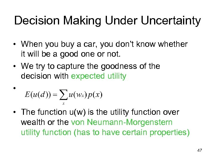Decision Making Under Uncertainty • When you buy a car, you don’t know whether it will be a good one or not. • We try to capture the goodness of the decision with expected utility • • The function u(w) is the utility function over wealth or the von Neumann-Morgenstern utility function (has to have certain properties) 47

• For our purposes, u(w) is any strictly increasing function u: [0, inf] • Decisions made under uncertainty can be thought of as choosing a lottery L over alternative levels of wealth wi where each level of wealth can be assigned a probability pi • Lottery L is a collection of pairs {{wi, pi)} • a lottery or gamble is simply a probability distribution over a known, finite set of outcomes. 48

Examples: • For the Derby betting pool, the set of outcomes A = {Giacomo wins, Closing Argument wins, Afleet Alex wins} • For the pharmaceutical company, the set of outcomes A = {Earn $500 million from patent, Earn $200 million from patent, Earn $0 from patent} • Each of these outcomes had a probability attached to it, and so we can define a simple lottery as a set of outcomes, A={a 1, a 2, . . . , an} each of which occurs with some known probability pi. 49

Compound Lottery • With two lotteries (having same set of alternatives) • L 1= {{wi, pi)} L 2 = {{w’i, p’i)} • we can combine: p. L 1 + (1 -p)L 2 is a compound lottery • We can then also construct compound lotteries, which are probability distributions over lotteries - i. e. , an outcome of a lottery may itself be another lottery. As a concrete example, imagine a Powerball lottery where the prize is yet another lottery ticket. Let G represent the set of all lotteries, or gambles, both simple and compound • Independence Axiom: If L 1 is preferred over L 2, then p. L 1+(1 -p)L 3 is preferred over p. L 2+(1 -p)L 3 50

Goals • Agent attempts to maximize its expected utility • Utility function ui of agent i is a mapping from outcomes to reals – Can be over a multi-dimensional outcome space – Incorporates agent’s risk attitude (allows quantitative tradeoffs) Lottery: a process, such as picking a name from a hat, through which goods are allocated randomly Lottery 1: $0. 5 M prob 1 Lottery 2: $1 M prob 0. 5 $0 prob 0. 5 Agent’s strategy is the choice of lottery ui Risk averse 1 Risk neutral 0. 5 0 0 Risk aversion => insurance companies Risk seeking 0. 5 1 M$ 51

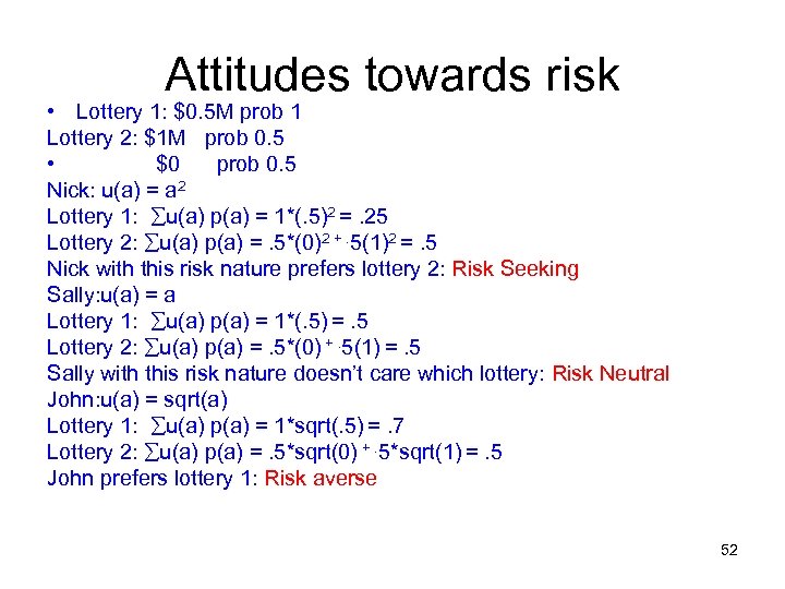Attitudes towards risk • Lottery 1: $0. 5 M prob 1 Lottery 2: $1 M prob 0. 5 • $0 prob 0. 5 Nick: u(a) = a 2 Lottery 1: u(a) p(a) = 1*(. 5)2 =. 25 Lottery 2: u(a) p(a) =. 5*(0)2 +. 5(1)2 =. 5 Nick with this risk nature prefers lottery 2: Risk Seeking Sally: u(a) = a Lottery 1: u(a) p(a) = 1*(. 5) =. 5 Lottery 2: u(a) p(a) =. 5*(0) +. 5(1) =. 5 Sally with this risk nature doesn’t care which lottery: Risk Neutral John: u(a) = sqrt(a) Lottery 1: u(a) p(a) = 1*sqrt(. 5) =. 7 Lottery 2: u(a) p(a) =. 5*sqrt(0) +. 5*sqrt(1) =. 5 John prefers lottery 1: Risk averse 52

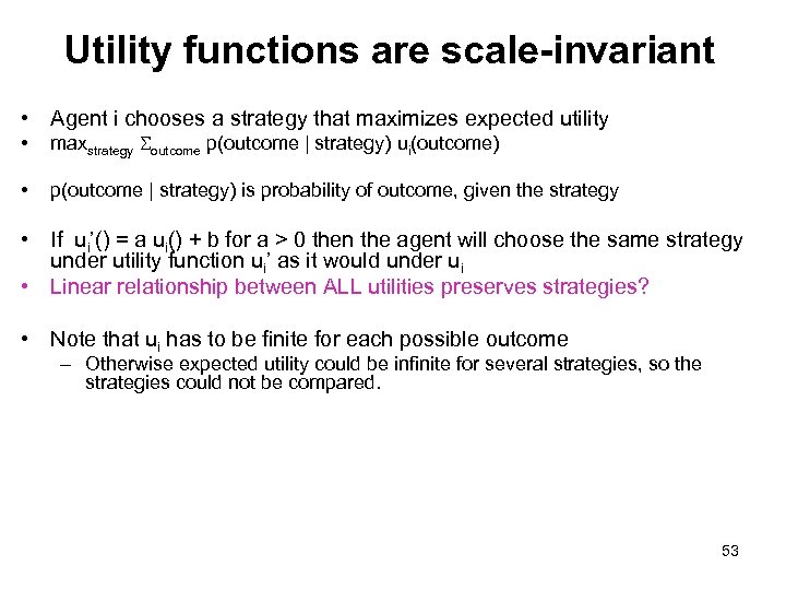Utility functions are scale-invariant • Agent i chooses a strategy that maximizes expected utility • maxstrategy Soutcome p(outcome | strategy) ui(outcome) • p(outcome | strategy) is probability of outcome, given the strategy • If ui’() = a ui() + b for a > 0 then the agent will choose the same strategy under utility function ui’ as it would under ui • Linear relationship between ALL utilities preserves strategies? • Note that ui has to be finite for each possible outcome – Otherwise expected utility could be infinite for several strategies, so the strategies could not be compared. 53

Full vs bounded rationality Full rationality Bounded rationality: How much can I afford to compute Descriptive vs. prescriptive theories of bounded rationality 54

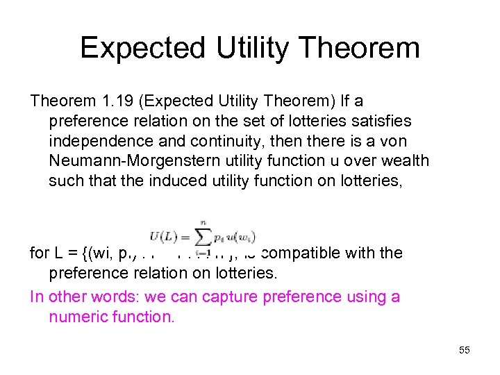Expected Utility Theorem 1. 19 (Expected Utility Theorem) If a preference relation on the set of lotteries satisfies independence and continuity, then there is a von Neumann-Morgenstern utility function u over wealth such that the induced utility function on lotteries, for L = {(wi, pi) : i = 1. . . n }, is compatible with the preference relation on lotteries. In other words: we can capture preference using a numeric function. 55

Utility Over Wealth • we could use the term Bernoulli Utility Function to refer to a decision-maker's utility over wealth - since it was Bernoulli who originally proposed the idea that people's internal, subjective value for an amount of money was not necessarily equal to the physical value of that money. • The term von Neumann-Morgenstern Utility Function, or Expected Utility Function is used to refer to a decision-maker's utility over lotteries, or gambles. 56

Risk Aversion and insurance • risk-averse individuals will always choose to insure valuable assets, since although the probability of a loss may be small, the potential loss of the asset itself would be so large that most people would rather pay small amounts of money as a premium for certain than risk the loss. On the other hand, insurance companies are risk-neutral, and earn their profits from the fact that the value of the premiums they receive is either greater than or equal to the expected value of the loss. 57

Example • Our discussion will assume that apart from knowning his own wealth, an individual making the decision to insure or not also knows for certain the probability of a loss or accident. Say you (a risk-averse consumer) have initial wealth w, and a von Neumann-Morgenstern utility function u(. ). You own a car of value L, and the probability of an accident which would total the car is p (we might imagine p as the current accident rate in the state where you live). If x is the amount of insurance you purchase, how much should x be? 58

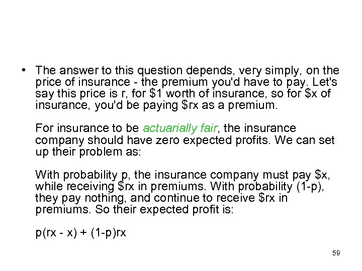• The answer to this question depends, very simply, on the price of insurance - the premium you'd have to pay. Let's say this price is r, for $1 worth of insurance, so for $x of insurance, you'd be paying $rx as a premium. For insurance to be actuarially fair, the insurance company should have zero expected profits. We can set up their problem as: With probability p, the insurance company must pay $x, while receiving $rx in premiums. With probability (1 -p), they pay nothing, and continue to receive $rx in premiums. So their expected profit is: p(rx - x) + (1 -p)rx 59

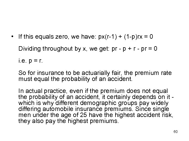• If this equals zero, we have: px(r-1) + (1 -p)rx = 0 Dividing throughout by x, we get: pr - p + r - pr = 0 i. e. p = r. So for insurance to be actuarially fair, the premium rate must equal the probability of an accident. In actual practice, even if the premium does not equal the probability of an accident, it certainly depends on it which is why different demographic groups pay widely differing automobile insurance premiums. Since single men under the age of 25 have the highest accident risk, they also pay the highest premiums. 60

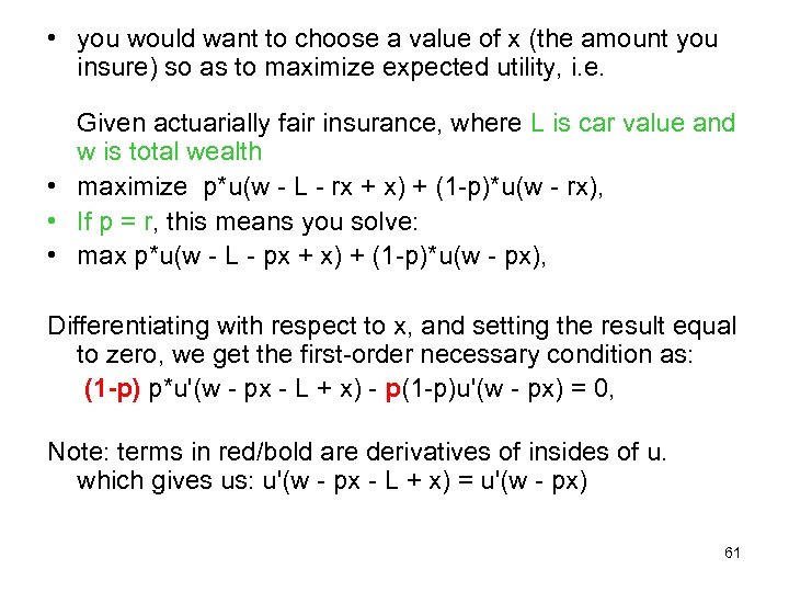• you would want to choose a value of x (the amount you insure) so as to maximize expected utility, i. e. Given actuarially fair insurance, where L is car value and w is total wealth • maximize p*u(w - L - rx + x) + (1 -p)*u(w - rx), • If p = r, this means you solve: • max p*u(w - L - px + x) + (1 -p)*u(w - px), Differentiating with respect to x, and setting the result equal to zero, we get the first-order necessary condition as: (1 -p) p*u'(w - px - L + x) - p(1 -p)u'(w - px) = 0, Note: terms in red/bold are derivatives of insides of u. which gives us: u'(w - px - L + x) = u'(w - px) 61

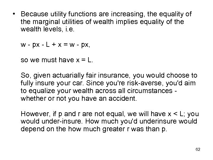• Because utility functions are increasing, the equality of the marginal utilities of wealth implies equality of the wealth levels, i. e. w - px - L + x = w - px, so we must have x = L. So, given actuarially fair insurance, you would choose to fully insure your car. Since you're risk-averse, you'd aim to equalize your wealth across all circumstances whether or not you have an accident. However, if p and r are not equal, we will have x < L; you would under-insure. How much you'd underinsure would depend on the how much greater r was than p. 62

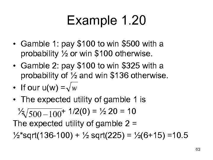Example 1. 20 • Gamble 1: pay $100 to win $500 with a probability ½ or win $100 otherwise. • Gamble 2: pay $100 to win $325 with a probability of ½ and win $136 otherwise. • If our u(w) = • The expected utility of gamble 1 is ½ + 1/2(0) = ½ 20 = 10 The expected utility of gamble 2 = ½*sqrt(136 -100) + ½ sqrt(225) = ½(6+15) =10. 5 63

• Of course, if the u(w)= w, Gamble 1 is better. • Individuals have different tolerance for risk. • An individual who ranks lotteries according to their expected value (rather than expected utility) is said to be risk neutral. In other words, an risk neutral individual who is offered $100 outright or a 50% chance of winning $200 will value the choices EQUALLY! 64

If the utility function over wealth is linear u(w) = aw + b the person is risk neutral • If the utility function is concave(line between points is under curve), the individual is risk averse. • If the utility function is convex(line between points is above curve), the individual is risk seeking. Note, gambling is like staying on the line as the two endpoints are picked with probability p or (1 -p). 65

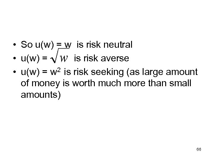• So u(w) = w is risk neutral • u(w) = is risk averse • u(w) = w 2 is risk seeking (as large amount of money is worth much more than small amounts) 66

Expected Utility Theory • describes behavior under uncertainty • If people are risk neutral or risk averse, they would never play the lottery or gamble (as return there is usually negative) • The expected value of Powerball lottery (if tickets cost $1 and jackpot is 7 million) is 7000000 * 1/85000000 -1(84999999/85000000) = -. 917647 67

But people do play powerball Why? • Loss is so small, people often ignore it. • If losses were larger, people may behave very differently. • People who buy lottery tickets may behave in very risk averse manner in other situation 68

Allais Paradox • In 1953, Maurice Allais published a paper regarding a survey he had conducted in 1952, with a hypothetical game. • Subjects "with good training in and knowledge of theory of probability, so that they could be considered to behave rationally", routinely violated the expected utility axioms. • The game itself and its results have now become famous as the "Allais Paradox". 69

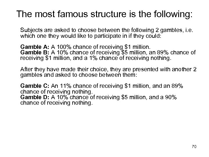The most famous structure is the following: Subjects are asked to choose between the following 2 gambles, i. e. which one they would like to participate in if they could: Gamble A: A 100% chance of receiving $1 million. Gamble B: A 10% chance of receiving $5 million, an 89% chance of receiving $1 million, and a 1% chance of receiving nothing. After they have made their choice, they are presented with another 2 gambles and asked to choose between them: Gamble C: An 11% chance of receiving $1 million, and an 89% chance of receiving nothing. Gamble D: A 10% chance of receiving $5 million, and a 90% chance of receiving nothing. 70

• This experiment has been conducted many, many times, and most people invariably prefer A to B, and D to C. So why is this a paradox? The expected value of A is $1 million, while the expected value of B is $1. 39 million. By preferring A to B, people are presumably maximizing expected utility, not expected value. By preferring A to B, we have the following expected utility relationship: u(1) > 0. 1 * u(5) + 0. 89 * u(1) + 0. 01 * u(0), i. e. 0. 11 * u(1) > 0. 1 * u(5) + 0. 1 * u(0) Adding 0. 89 * u(0) to each side, we get: 0. 11 * u(1) + 0. 89 * u(0) > 0. 1 * u(5) + 0. 90 * u(0), implying that an expected utility maximizer must prefer C to D. Of course, the expected value of C is $110, 000, while the expected value of D is $500, 000, so if people were maximizing expected value, they should in fact prefer D to C. However, their choice in the first stage is inconsistent with their choice in the second stage, and herein lies the paradox. From the Von Neumann-Morgenstern axioms, the substitution axiom is the one that is clearly violated. The probability of receiving $5 million is the same in both B and D. 71

Ellsberg Paradox In 1961, Daniel Ellsberg published the results of a hypothetical experiment he had conducted, which, to many, constitutes an even worse violation of the expected utility axioms than the Allais Paradox. Ellsberg's subjects in his thought experiment seemed to run the gamut of noted economists of the time, from Gerard Debreu to Paul Samuelson and Howard Raiffa. 72

The Experiment • • • Suppose there are two large pots, each containing black and red balls. The first pot contains 50 black and 50 red balls. The second pot also contains 100 balls but the mix between red and black balls is unknown. You win $500 if you draw a red ball. Which pot will you choose? You are most likely to choose the first pot, as did the people who were part of Ellsberg's experiment. Why? You know there is a 50 per cent chance of getting a red ball if you choose the first pot. The probability of drawing a red ball from the second pot is not known. Next, you are offered $500 to draw a black ball. What will you do? Chances are you will still select the first pot! That is the paradox. The first time you chose the first pot because you thought the other one had fewer red balls. Logically, it meant that you thought there were more black balls in the second pot. So, you should have chosen this pot in the second experiment —$500 for a black ball. 73

• After a series of such experiments, Daniel Ellsberg concluded that people behave this way because they prefer to avoid ambiguity. In the above case, choosing black or red ball from the second pot was ambiguous, as the mix was not known. • The Ellsberg Paradox essentially states that we treat ambiguous choices as risky. This has been cited as one of the reasons for the high returns in the stock market. Stock price movements are ambiguous. So we treat the stock market as risky and demand high returns. 74