Challenges and Opportunities in Using Automatic Differentiation with

Challenges and Opportunities in Using Automatic Differentiation with Object. Oriented Toolkits for Scientific Computing Paul Hovland (Argonne National Laboratory) Steven Lee (Lawrence Livermore National Laboratory) Lois Mc. Innes (ANL) Boyana Norris (ANL) Barry Smith (ANL) The Computational Differentiation Project at Argonne National Laboratory

Acknowledgments l l l Jason Abate Satish Balay Steve Benson Peter Brown Omar Ghattas Lisa Grignon William Gropp Alan Hindmarsh David Keyes Jorge Moré Linda Petzold Widodo Samyono

Outline l l l Intro to AD Survey of Toolkits Q Sens. PVODE Q PETSc Q TAO Using AD with Toolkits Q Toolkit Level Q Parallel Function Level Q Subdomain Level Q Element/Vertex Function Level Experimental Results Conclusions and Expectations

Automatic Differentiation l l Technique for augmenting code for computing a function with code for computing derivatives Analytic differentiation of elementary operations/functions, propagation by chain rule Can be implemented using source transformation or operator overloading Two main modes Q Forward: propagates derivatives from independent to dependent variables Q Reverse (adjoint): propagates derivatives from dependent to independent variables

Comparison of Methods l l l Finite Differences Q Advantages: cheap Jv, easy Q Disadvantages: inaccurate (not robust) Hand Differentiation Q Advantages: accurate; cheap Jv, JTv, Hv, … Q Disadvantages: hard; difficult to maintain consistency Automatic Differentiation Q Advantages: cheap JTv, Hv; easy? Q Disadvantages: Jv costs ~2 function evals; hard?

PVODE: Parallel ODE-IVP solver l Algorithm developers: Hindmarsh, Byrne, Brown and Cohen l ODE Initial-Value Problems l Stiff and non-stiff integrators l Written in C l MPI calls for communication

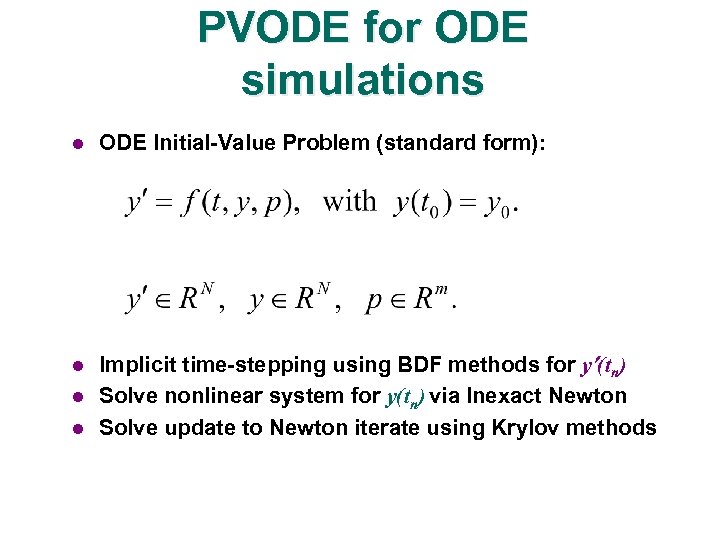PVODE for ODE simulations l ODE Initial-Value Problem (standard form): l Implicit time-stepping using BDF methods for y (tn) Solve nonlinear system for y(tn) via Inexact Newton Solve update to Newton iterate using Krylov methods l l

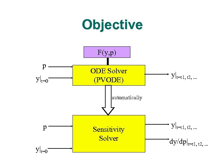Objective F(y, p) p y|t=0 ODE Solver (PVODE) y|t=t 1, t 2, . . . automatically p y|t=0 Sensitivity Solver y|t=t 1, t 2, . . . dy/dp|t=t 1, t 2, . . .

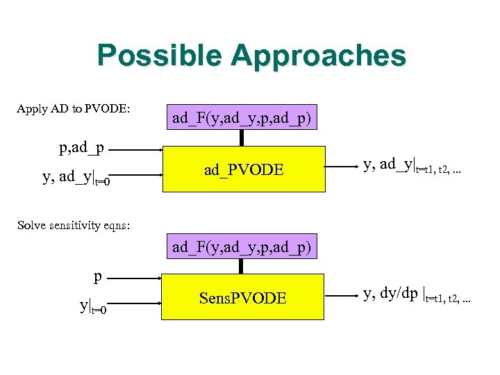Possible Approaches Apply AD to PVODE: ad_F(y, ad_y, p, ad_p) p, ad_p y, ad_y|t=0 ad_PVODE y, ad_y|t=t 1, t 2, . . . Solve sensitivity eqns: ad_F(y, ad_y, p, ad_p) p y|t=0 Sens. PVODE y, dy/dp |t=t 1, t 2, . . .

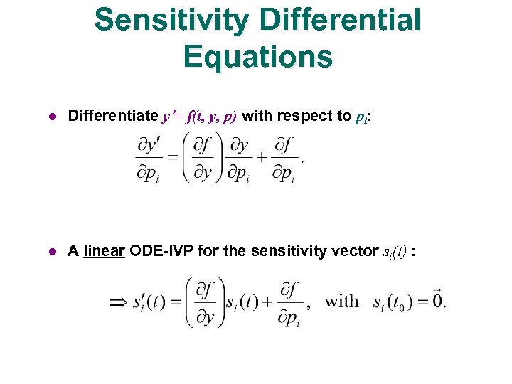Sensitivity Differential Equations l Differentiate y = f(t, y, p) with respect to pi: l A linear ODE-IVP for the sensitivity vector si(t) :

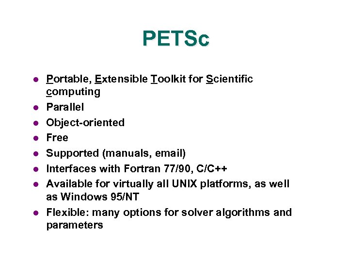PETSc l l l l Portable, Extensible Toolkit for Scientific computing Parallel Object-oriented Free Supported (manuals, email) Interfaces with Fortran 77/90, C/C++ Available for virtually all UNIX platforms, as well as Windows 95/NT Flexible: many options for solver algorithms and parameters

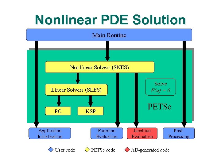Nonlinear PDE Solution Main Routine Nonlinear Solvers (SNES) Linear Solvers (SLES) PC Application Initialization User code Solve F(u) = 0 PETSc KSP Function Evaluation PETSc code Jacobian Evaluation Post. Processing AD-generated code

TAO The process of nature by which all things change and which is to be followed for a life of harmony The Right Way Toolkit for advanced optimization l l Object-oriented techniques Component-based (CCA) interaction Leverage existing parallel computing infrastructure Reuse of external toolkits

TAO Goals l Portability l Performance l Scalable parallelism l An interface independent of architecture

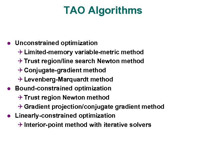TAO Algorithms l l l Unconstrained optimization Q Limited-memory variable-metric method Q Trust region/line search Newton method Q Conjugate-gradient method Q Levenberg-Marquardt method Bound-constrained optimization Q Trust region Newton method Q Gradient projection/conjugate gradient method Linearly-constrained optimization Q Interior-point method with iterative solvers

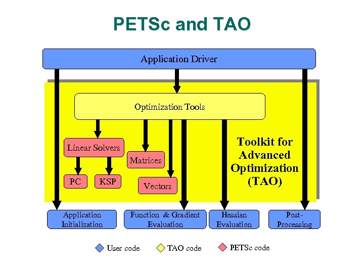PETSc and TAO Application Driver Optimization Tools Linear Solvers Matrices PC KSP Application Initialization Vectors Function & Gradient Evaluation User code TAO code Toolkit for Advanced Optimization (TAO) Hessian Evaluation PETSc code Post. Processing

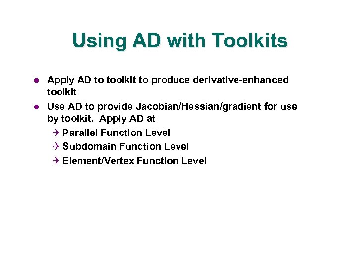Using AD with Toolkits l l Apply AD to toolkit to produce derivative-enhanced toolkit Use AD to provide Jacobian/Hessian/gradient for use by toolkit. Apply AD at Q Parallel Function Level Q Subdomain Function Level Q Element/Vertex Function Level

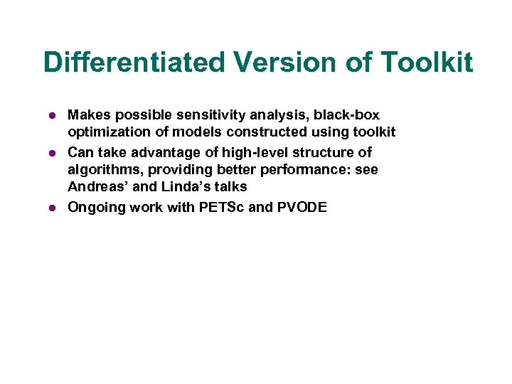Differentiated Version of Toolkit l l l Makes possible sensitivity analysis, black-box optimization of models constructed using toolkit Can take advantage of high-level structure of algorithms, providing better performance: see Andreas’ and Linda’s talks Ongoing work with PETSc and PVODE

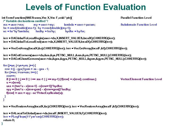Levels of Function Evaluation int Form. Function(SNES snes, Vec X, Vec F, void *ptr){ /* Variable declarations omitted */ mx = user->mx; my = user->my; lambda = user->param; hx = one/(double)(mx-1); hy = one/(double)(my-1); sc = hx*hy*lambda; hxdhy = hx/hy; hydhx = hy/hx; Parallel Function Level Subdomain Function Level ierr = DAGlobal. To. Local. Begin(user->da, X, INSERT_VALUES, local. X); CHKERRQ(ierr); ierr = DAGlobal. To. Local. End(user->da, X, INSERT_VALUES, local. X); CHKERRQ(ierr); ierr = Vec. Get. Array(local. X, &x); CHKERRQ(ierr); ierr = Vec. Get. Array(local. F, &f); CHKERRQ(ierr); ierr = DAGet. Corners(user->da, &xs, &ys, PETSC_NULL, &xm, &ym, PETSC_NULL); CHKERRQ(ierr); ierr = DAGet. Ghost. Corners(user->da, &gxs, &gys, PETSC_NULL, &gxm, &gym, PETSC_NULL); CHKERRQ(ierr); for (j=ys; jda, local. F, INSERT_VALUES, F); CHKERRQ(ierr); ierr = PLog. Flops(11*ym*xm); CHKERRQ(ierr); return 0; }

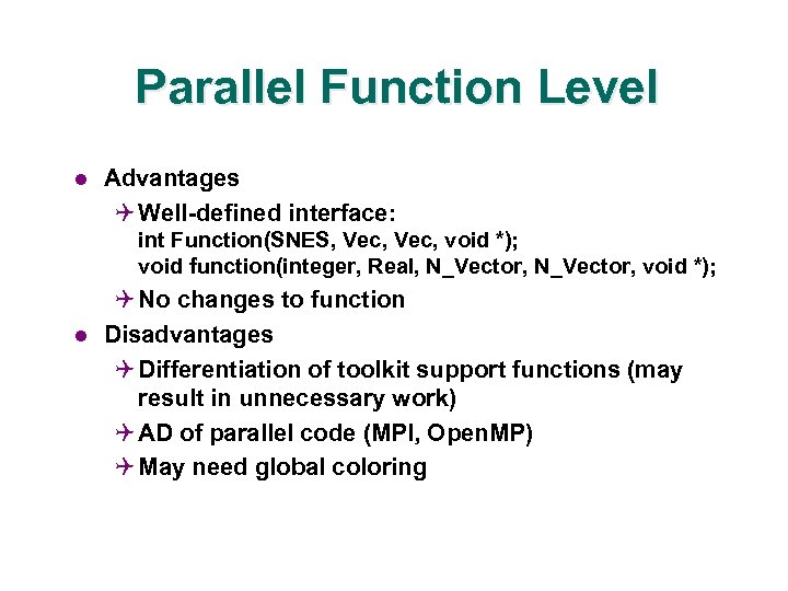Parallel Function Level l Advantages Q Well-defined interface: int Function(SNES, Vec, void *); void function(integer, Real, N_Vector, void *); l Q No changes to function Disadvantages Q Differentiation of toolkit support functions (may result in unnecessary work) Q AD of parallel code (MPI, Open. MP) Q May need global coloring

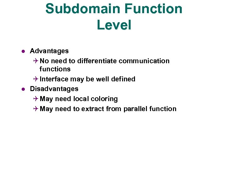Subdomain Function Level l l Advantages Q No need to differentiate communication functions Q Interface may be well defined Disadvantages Q May need local coloring Q May need to extract from parallel function

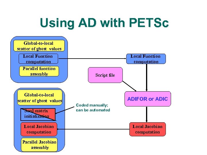Using AD with PETSc Global-to-local scatter of ghost values Local Function computation Parallel function assembly Local Function computation Script file Global-to-local scatter of ghost values Seed matrix initialization Local Jacobian computation Parallel Jacobian assembly ADIFOR or ADIC Coded manually; can be automated Local Jacobian computation

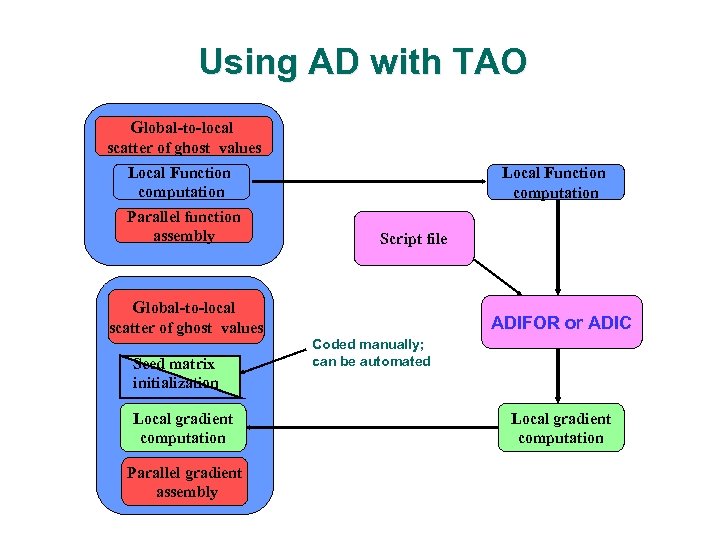Using AD with TAO Global-to-local scatter of ghost values Local Function computation Parallel function assembly Local Function computation Script file Global-to-local scatter of ghost values Seed matrix initialization Local gradient computation Parallel gradient assembly ADIFOR or ADIC Coded manually; can be automated Local gradient computation

Element/Vertex Function Level l l Advantages Q Reduced memory requirements Q No need for matrix coloring Disadvantages Q May be difficult to decompose function to this level (boundary conditions, other special cases) Q Decomposition to this level may impede efficiency

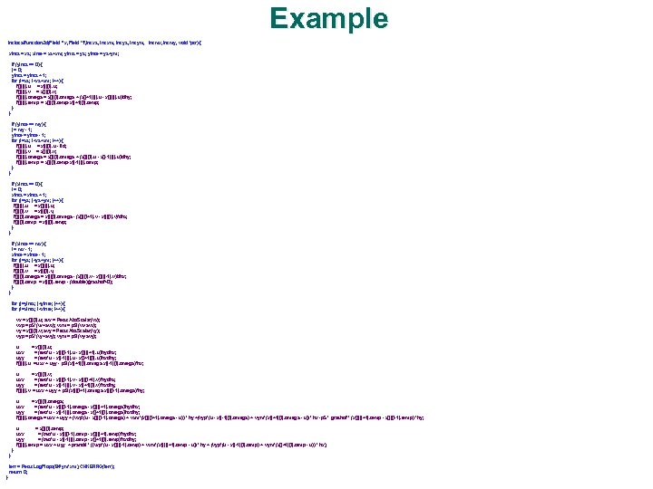Example int localfunction 2 d(Field **x, Field **f, int xs, int xm, int ys, int ym, int mx, int my, void *ptr) { xints = xs; xinte = xs+xm; yints = ys; yinte = ys+ym; if (yints == 0) { j = 0; yints = yints + 1; for (i=xs; i0); } } for (j=yints; j

Experimental Results l l Toolkit Level – Differentiated PETSc Linear Solver Parallel Nonlinear Function Level – Sens. PVODE Local Subdomain Function Level Q PETSc Q TAO Element Function Level – PETSc

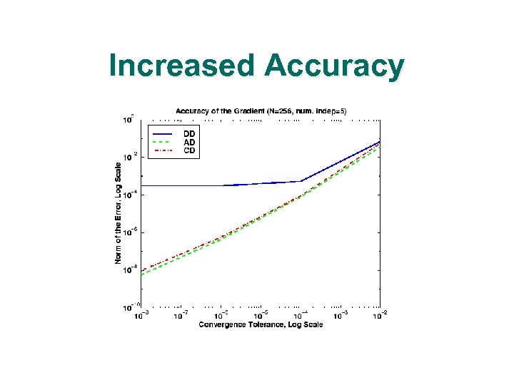
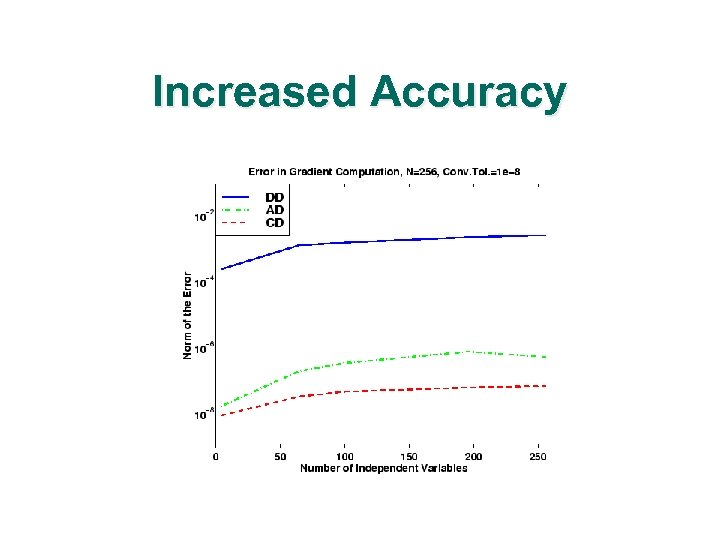
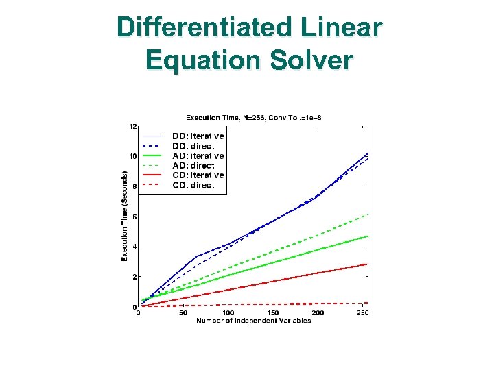Differentiated Linear Equation Solver

Increased Accuracy

Increased Accuracy

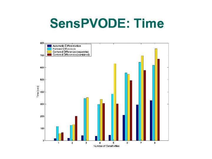
Sens. PVODE: Problem l l l Diurnl kinetics advection-diffusion equation 100 x 100 structured grid 16 processors of a Linux cluster with 550 MHz processors and Myrinet interconnect

Sens. PVODE: Time

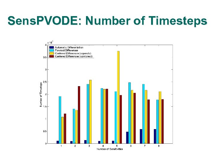Sens. PVODE: Number of Timesteps

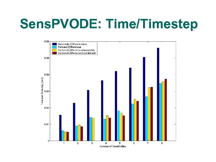Sens. PVODE: Time/Timestep

PETSc Applications l l Toy problems Q Solid fuel ignition: finite difference discretization; Fortran & C variants; differentiated using ADIFOR, ADIC Q Driven cavity: finite difference discretization; C implementation; differentiated using ADIC Euler code Q Based on legacy F 77 code from D. Whitfield (MSU) Q Finite volume discretization Q Up to 1, 121, 320 unknowns Q Mapped C-H grid Q Fully implicit steady-state Q Tools: SNES, DA, ADIFOR

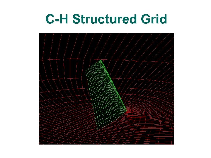C-H Structured Grid

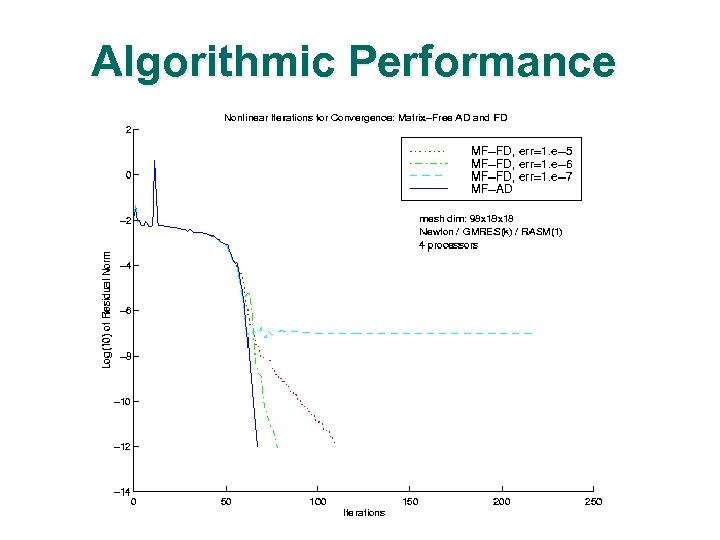Algorithmic Performance

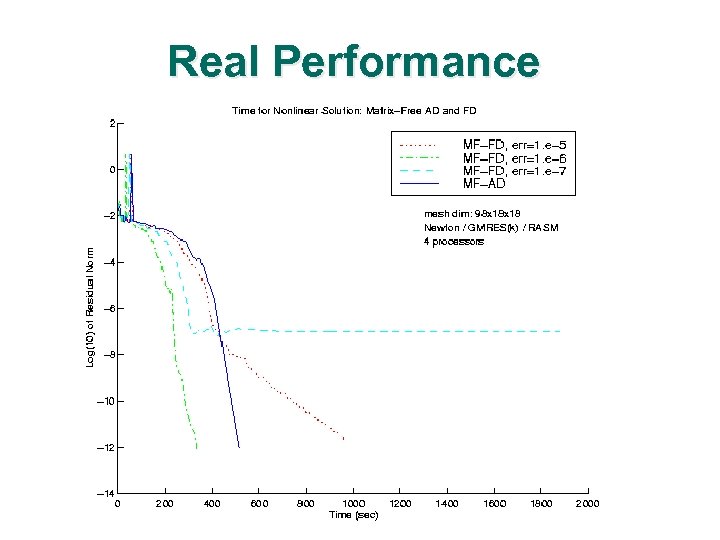Real Performance

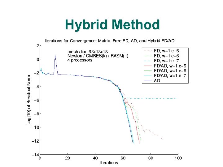Hybrid Method

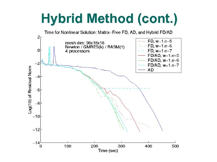Hybrid Method (cont. )

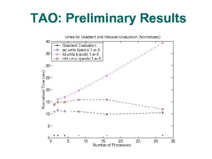TAO: Preliminary Results

For More Information l PETSc: http: //www. mcs. anl. gov/petsc/ TAO: http: //www. mcs. anl. gov/tao/ l Automatic Differentiation at Argonne l Q http: //www. mcs. anl. gov/autodiff/ Q ADIFOR: http: //www. mcs. anl. gov/adifor/ Q ADIC: http: //www. mcs. anl. gov/adic/ l http: //www. autodiff. org

10 challenges for PDE optimization algorithms Problem size 2. Efficiency vs. intrusiveness 3. “Physics-based” globalizations 4. Inexact PDE solvers 5. Approximate Jacobians 6. Implicitly-defined PDE residuals 7. Non-smooth solutions 8. Pointwise inequality constraints 9. Scalability of adjoint methods to large numbers of inequalities 10. Time-dependent PDE optimization 1.

7. Non-smoothness l l PDE residual may not depend smoothly on state variables (maybe not even continuously) Q Solution-adaptivity Q Discontinuity-capturing, front-tracking Q Subgrid-scale models Q Material property evaluation Q Contact problems Q Elasto(visco)plasticity PDE residual may not depend smoothly or continuously on decision variables Q Solid modeler- and mesh generator-induced