CH 20 — AGGREGATE DEMAND SUPPLY Aggregate Demand

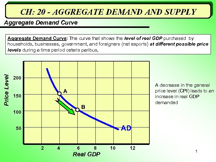CH: 20 - AGGREGATE DEMAND SUPPLY Aggregate Demand Curve Price Level Aggregate Demand Curve: The curve that shows the level of real GDP purchased by households, businesses, government, and foreigners (net exports) at different possible price levels during a time period ceteris paribus, 200 A decrease in the general price level (CPI) leads to an increase in real GDP demanded A 150 B 100 AD 50 2 4 6 8 Real GDP 10 12 1

CH: 20 - AGGREGATE DEMAND SUPPLY Shape of the Aggregate Demand Curve The reasons for the downward slope of an AD curve include: § The Real Balances or Wealth Effect § The Interest Rate Effect § The Net Exports Effect 2

CH: 20 - AGGREGATE DEMAND SUPPLY Shape of the Aggregate Demand Curve The Real Balances (Wealth) Effect: Consumers spend more on goods and services because lower prices make their dollars more valuable Example: • Suppose you have $1, 000 to buy 10 weeks worth of groceries. • If price falls by 20%, $1, 000 will now buy enough groceries for 12 weeks. • Knowing this makes you more likely to spend money on something stupid 3

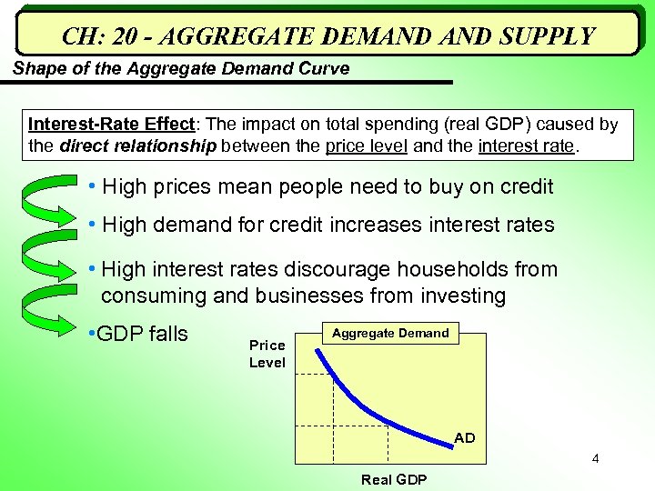CH: 20 - AGGREGATE DEMAND SUPPLY Shape of the Aggregate Demand Curve Interest-Rate Effect: The impact on total spending (real GDP) caused by the direct relationship between the price level and the interest rate. • High prices mean people need to buy on credit • High demand for credit increases interest rates • High interest rates discourage households from consuming and businesses from investing • GDP falls Price Level Aggregate Demand AD 4 Real GDP

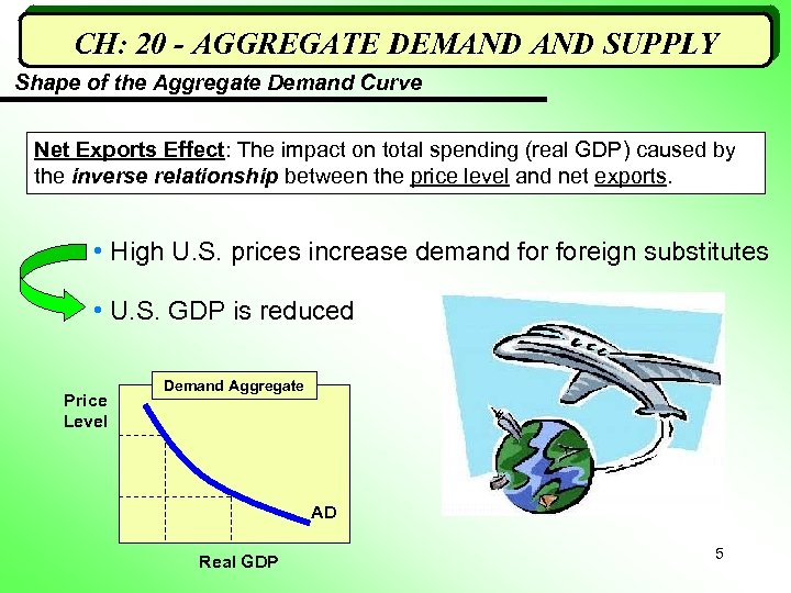CH: 20 - AGGREGATE DEMAND SUPPLY Shape of the Aggregate Demand Curve Net Exports Effect: The impact on total spending (real GDP) caused by the inverse relationship between the price level and net exports. • High U. S. prices increase demand foreign substitutes • U. S. GDP is reduced Price Level Demand Aggregate AD Real GDP 5

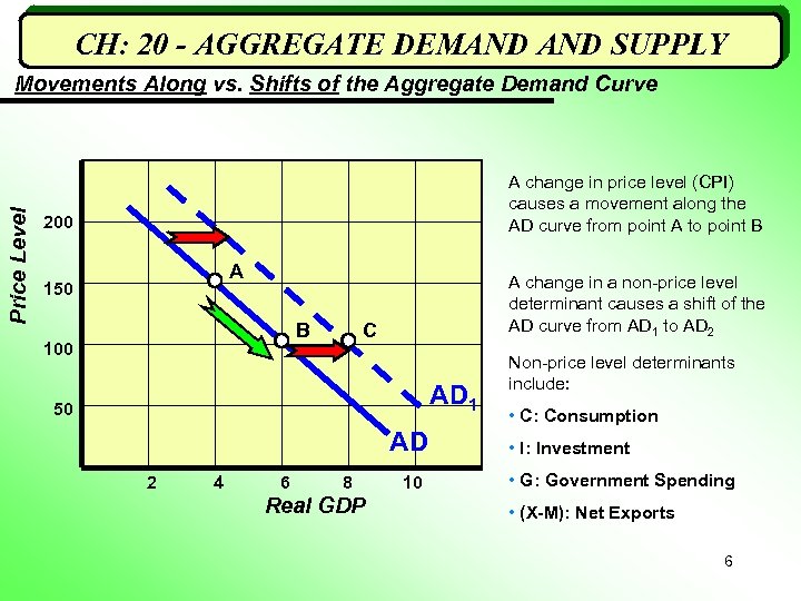CH: 20 - AGGREGATE DEMAND SUPPLY Price Level Movements Along vs. Shifts of the Aggregate Demand Curve A change in price level (CPI) causes a movement along the AD curve from point A to point B 200 A 150 B 100 A change in a non-price level determinant causes a shift of the AD curve from AD 1 to AD 2 C AD 1 50 AD 2 4 6 8 Real GDP 10 Non-price level determinants include: • C: Consumption • I: Investment • G: Government Spending • (X-M): Net Exports 6

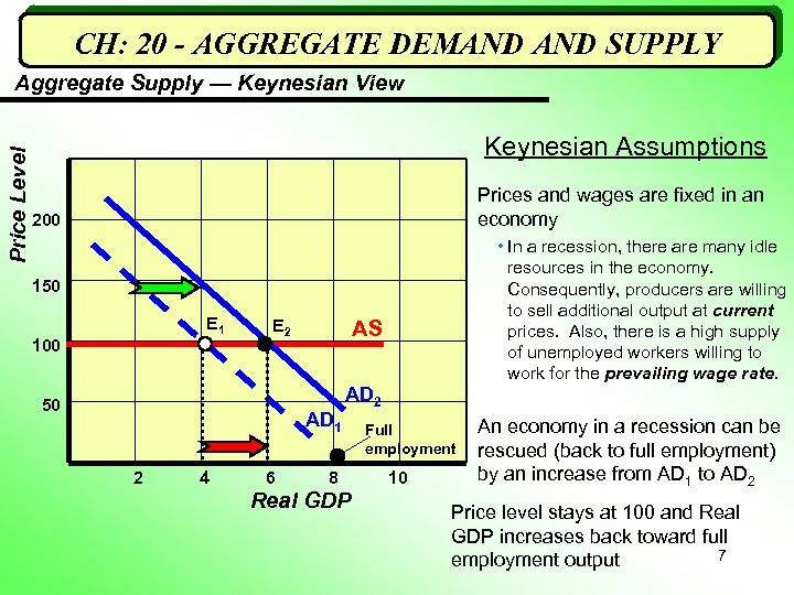CH: 20 - AGGREGATE DEMAND SUPPLY Price Level Aggregate Supply — Keynesian View Keynesian Assumptions Prices and wages are fixed in an economy 200 • In a recession, there are many idle resources in the economy. Consequently, producers are willing to sell additional output at current prices. Also, there is a high supply of unemployed workers willing to work for the prevailing wage rate. 150 E 1 100 E 2 50 AS AD 1 2 4 6 AD 2 8 Real GDP Full employment 10 An economy in a recession can be rescued (back to full employment) by an increase from AD 1 to AD 2 Price level stays at 100 and Real GDP increases back toward full 7 employment output

CH: 20 - AGGREGATE DEMAND SUPPLY Aggregate Supply — Keynesian View Idle resources are reemployed during a recession to increase GDP without driving up price level 8

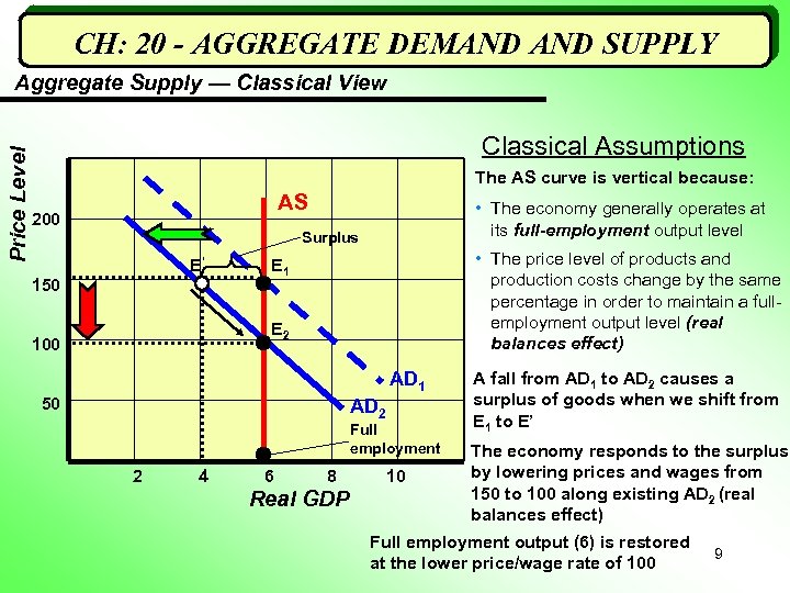CH: 20 - AGGREGATE DEMAND SUPPLY Price Level Aggregate Supply — Classical View Classical Assumptions The AS curve is vertical because: AS 200 • The economy generally operates at its full-employment output level Surplus E’ 150 • The price level of products and production costs change by the same percentage in order to maintain a fullemployment output level (real balances effect) E 1 E 2 100 AD 1 50 AD 2 Full employment 2 4 6 8 Real GDP 10 A fall from AD 1 to AD 2 causes a surplus of goods when we shift from E 1 to E’ The economy responds to the surplus by lowering prices and wages from 150 to 100 along existing AD 2 (real balances effect) Full employment output (6) is restored at the lower price/wage rate of 100 9

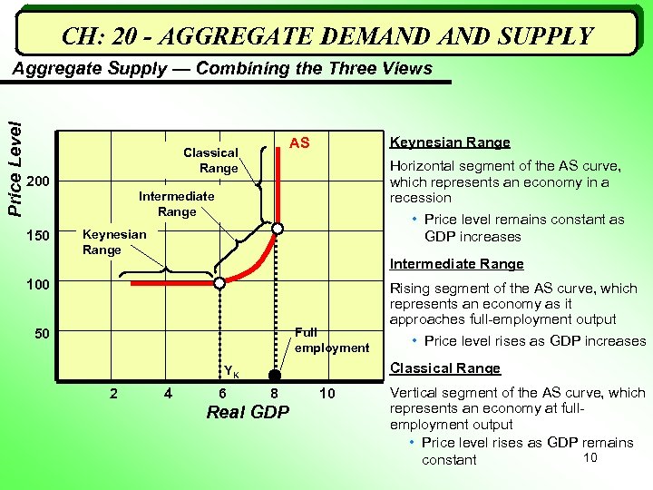CH: 20 - AGGREGATE DEMAND SUPPLY Price Level Aggregate Supply — Combining the Three Views 200 Keynesian Range AS Classical Range Horizontal segment of the AS curve, which represents an economy in a recession Intermediate Range 150 • Price level remains constant as GDP increases Keynesian Range Intermediate Range 100 Full employment 50 4 6 • Price level rises as GDP increases Classical Range YK 2 Rising segment of the AS curve, which represents an economy as it approaches full-employment output 8 Real GDP 10 Vertical segment of the AS curve, which represents an economy at fullemployment output • Price level rises as GDP remains 10 constant

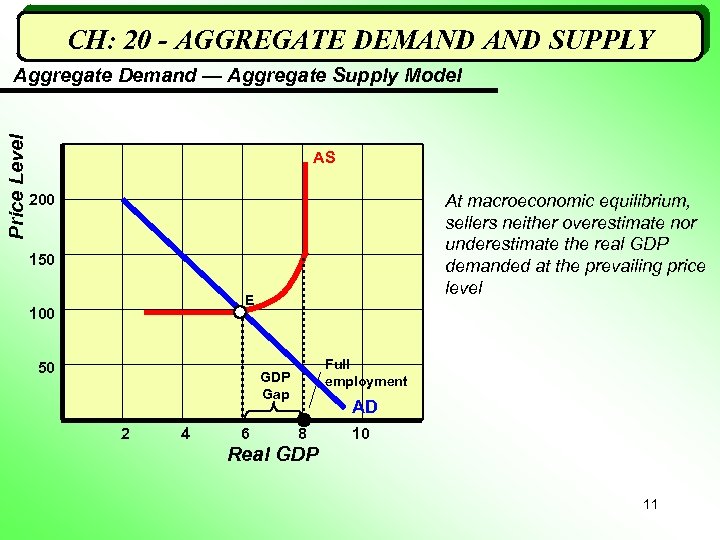CH: 20 - AGGREGATE DEMAND SUPPLY Price Level Aggregate Demand — Aggregate Supply Model AS 200 At macroeconomic equilibrium, sellers neither overestimate nor underestimate the real GDP demanded at the prevailing price level 150 E 100 50 Full employment GDP Gap 2 4 6 AD 8 10 Real GDP 11

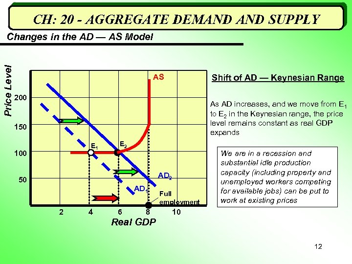CH: 20 - AGGREGATE DEMAND SUPPLY Price Level Changes in the AD — AS Model AS Shift of AD — Keynesian Range 200 As AD increases, and we move from E 1 to E 2 in the Keynesian range, the price level remains constant as real GDP expands 150 E 1 100 E 2 AD 2 50 AD 1 2 4 6 8 Full employment We are in a recession and substantial idle production capacity (including property and unemployed workers competing for available jobs) can be put to work at existing prices 10 Real GDP 12

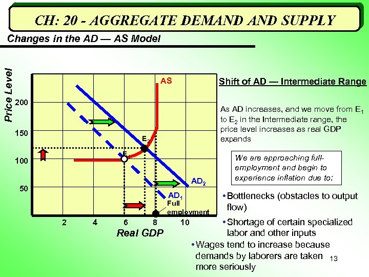CH: 20 - AGGREGATE DEMAND SUPPLY Price Level Changes in the AD — AS Model AS Shift of AD — Intermediate Range 200 150 As AD increases, and we move from E 1 to E 2 in the Intermediate range, the price level increases as real GDP expands E 2 E 1 100 AD 2 50 AD 1 Full employment 2 4 6 8 Real GDP 10 We are approaching fullemployment and begin to experience inflation due to: • Bottlenecks (obstacles to output flow) • Shortage of certain specialized labor and other inputs • Wages tend to increase because demands by laborers are taken 13 more seriously

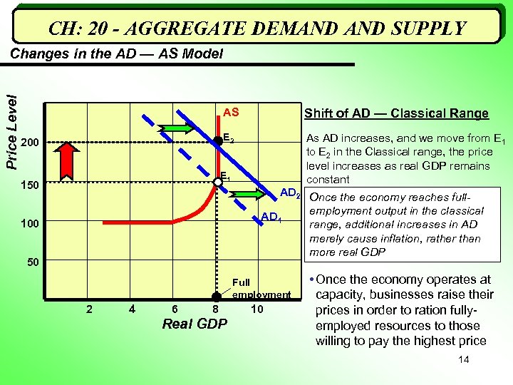CH: 20 - AGGREGATE DEMAND SUPPLY Price Level Changes in the AD — AS Model AS E 2 200 Shift of AD — Classical Range As AD increases, and we move from E 1 to E 2 in the Classical range, the price level increases as real GDP remains constant E 1 150 AD 2 Once the economy reaches fullemployment output in the classical AD 1 range, additional increases in AD merely cause inflation, rather than more real GDP 100 50 Full employment 2 4 6 8 Real GDP 10 • Once the economy operates at capacity, businesses raise their prices in order to ration fullyemployed resources to those willing to pay the highest price 14

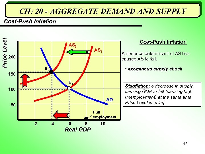CH: 20 - AGGREGATE DEMAND SUPPLY Price Level Cost-Push Inflation AS 2 AS 1 A nonprice determinant of AS has caused AS to fall. 200 • exogenous supply shock E 2 150 E 1 100 AD 50 Stagflation: a decrease in supply causing GDP to fall (causing high unemployment) at the same time Price Level is rising Full employment 2 4 6 8 10 Real GDP 15

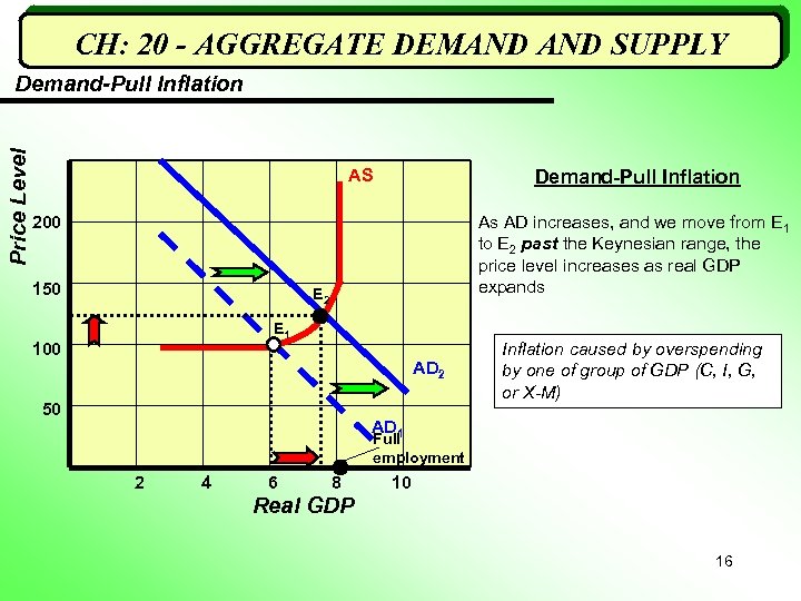CH: 20 - AGGREGATE DEMAND SUPPLY Price Level Demand-Pull Inflation AS Demand-Pull Inflation 200 150 As AD increases, and we move from E 1 to E 2 past the Keynesian range, the price level increases as real GDP expands E 2 E 1 100 AD 2 50 Inflation caused by overspending by one of group of GDP (C, I, G, or X-M) AD 1 Full employment 2 4 6 8 10 Real GDP 16

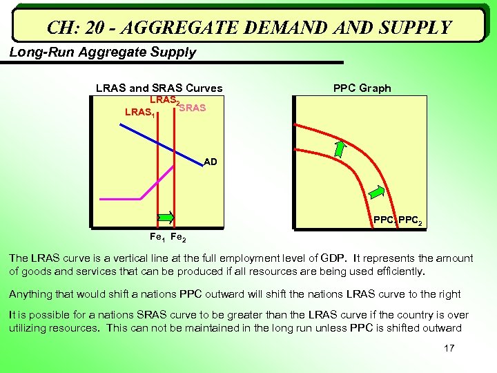CH: 20 - AGGREGATE DEMAND SUPPLY Long-Run Aggregate Supply LRAS and SRAS Curves PPC Graph LRAS 2 SRAS LRAS 1 AD PPC 1 PPC 2 Fe 1 Fe 2 The LRAS curve is a vertical line at the full employment level of GDP. It represents the amount of goods and services that can be produced if all resources are being used efficiently. Anything that would shift a nations PPC outward will shift the nations LRAS curve to the right It is possible for a nations SRAS curve to be greater than the LRAS curve if the country is over utilizing resources. This can not be maintained in the long run unless PPC is shifted outward 17