Ch 18 Extensions of Demand Supply

Ch 18. Extensions of Demand & Supply

A. Price elasticity of demand – responsiveness (sensitivity) of consumers to a price change ($ Δ). LAW OF DEMAND: $ = Purchases Three ideas: l Price elasticity l Cross elasticity – buying response of consumers of one product when the price of another product changes. l Income elasticity – the buying response of consumers when their income changes.

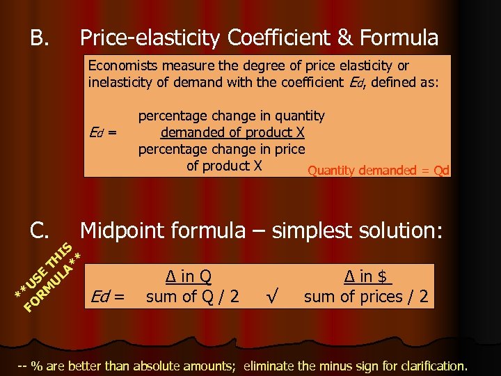B. Price-elasticity Coefficient & Formula Economists measure the degree of price elasticity or inelasticity of demand with the coefficient Ed, defined as: Ed = Midpoint formula – simplest solution: * FO *U R SE M T U H LA IS ** C. percentage change in quantity demanded of product X percentage change in price of product X Quantity demanded = Qd Ed = Δ in Q sum of Q / 2 √ Δ in $ sum of prices / 2 -- % are better than absolute amounts; eliminate the minus sign for clarification.

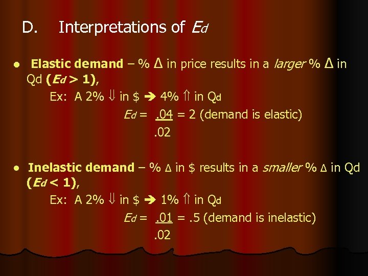D. l Interpretations of Ed Elastic demand – % Δ in price results in a larger % Δ in Qd (Ed > 1), Ex: A 2% in $ 4% in Qd Ed =. 04 = 2 (demand is elastic). 02 ● Inelastic demand – % Δ in $ results in a smaller % Δ in Qd (Ed < 1), Ex: A 2% in $ 1% in Qd Ed =. 01 =. 5 (demand is inelastic). 02

l Unit elasticity – % Δ in $ and the resulting % Δ in Qd are the same (Ed = 1), Ex: A 2% in $ 2% in Qd Ed =. 02 = 1 (unit elasticity). 02 ● Perfectly inelastic (rare) – coefficient is zero due to consumers being unresponsive to a $ Δ.

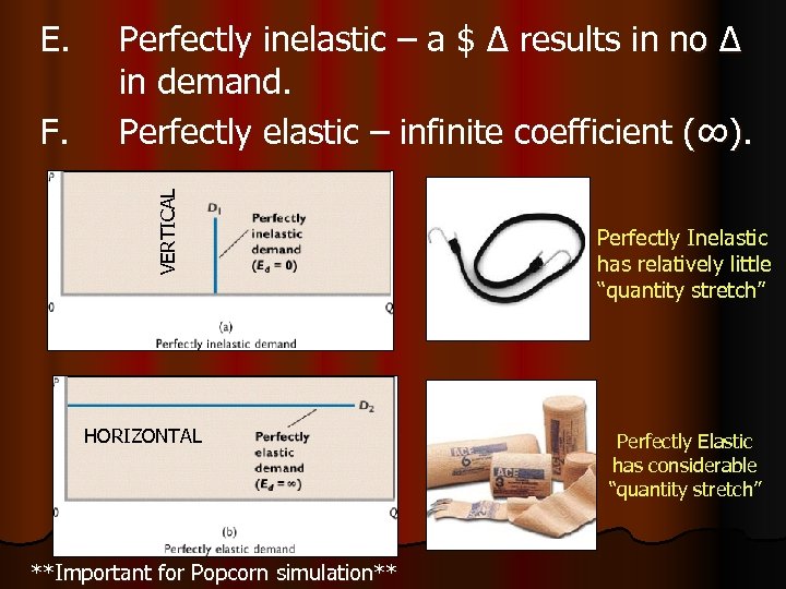E. VERTICAL F. Perfectly inelastic – a $ Δ results in no Δ in demand. Perfectly elastic – infinite coefficient (∞). HORIZONTAL **Important for Popcorn simulation** Perfectly Inelastic has relatively little “quantity stretch” Perfectly Elastic has considerable “quantity stretch”

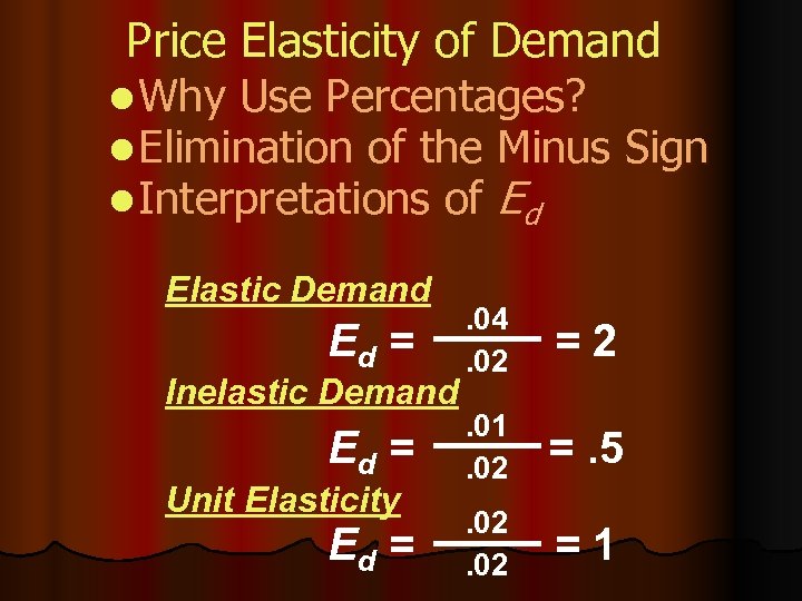Price Elasticity of Demand l Why Use Percentages? l Elimination of the Minus Sign l Interpretations of Ed Elastic Demand Ed = . 04. 02 =2 Ed = . 01. 02 =. 5 Ed = . 02 =1 Inelastic Demand Unit Elasticity

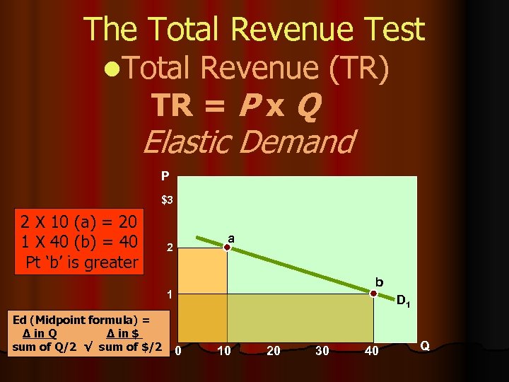The Total Revenue Test l. Total Revenue (TR) TR = P x Q Elastic Demand P $3 2 X 10 (a) = 20 1 X 40 (b) = 40 Pt ‘b’ is greater a 2 b 1 Ed (Midpoint formula) = Δ in Q Δ in $ sum of Q/2 √ sum of $/2 D 1 0 10 20 30 40 Q

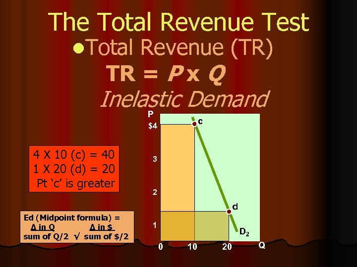The Total Revenue Test l. Total Revenue (TR) TR = P x Q Inelastic Demand P c $4 4 X 10 (c) = 40 1 X 20 (d) = 20 Pt ‘c’ is greater 3 2 d Ed (Midpoint formula) = Δ in Q Δ in $ sum of Q/2 √ sum of $/2 1 D 2 0 10 20 Q

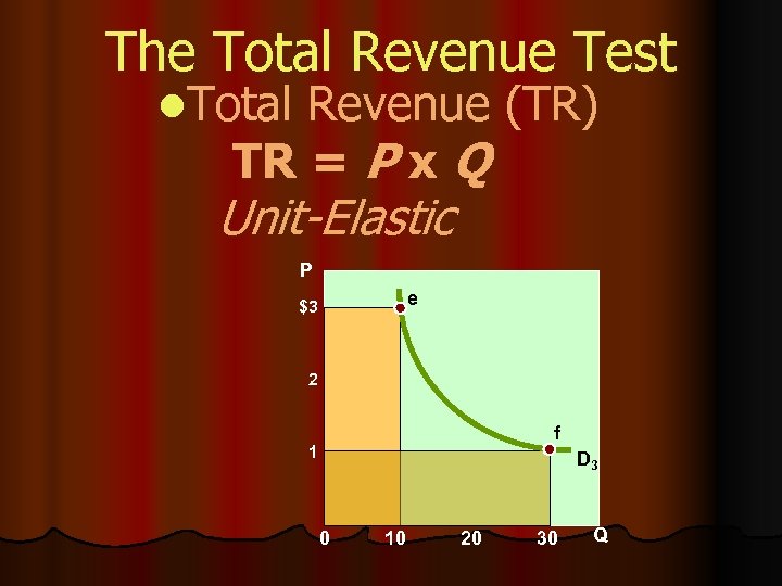The Total Revenue Test l. Total Revenue (TR) TR = P x Q Unit-Elastic P e $3 2 f 1 D 3 0 10 20 30 Q

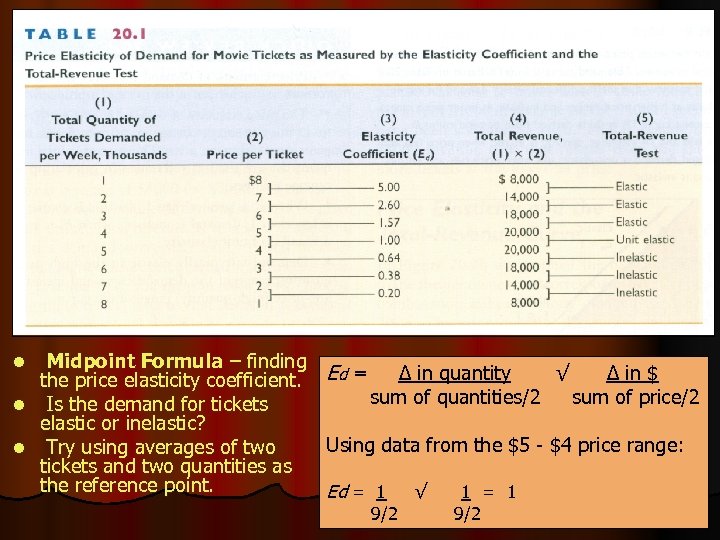Midpoint Formula – finding Δ in quantity √ Δ in $ the price elasticity coefficient. Ed = sum of quantities/2 sum of price/2 l Is the demand for tickets elastic or inelastic? Using data from the $5 - $4 price range: l Try using averages of two tickets and two quantities as the reference point. Ed = 1 √ 1 = 1 l 9/2

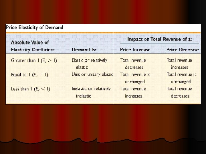
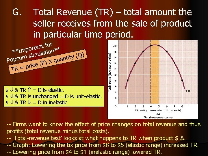G. Total Revenue (TR) – total amount the seller receives from the sale of product in particular time period. for rtant o **Imp mulation** i Q) corn s ntity ( Pop qua (P) X e = pric TR $ & TR = D is elastic. $ & TR is unchanged = D is unit-elastic. $ & TR = D in inelastic -- Firms want to know the effect of price changes on total revenue and thus profits (total revenue minus total costs). -- ‘Total-revenue test’ looks at what happens to TR when product $ Δ. -- Graph: Lowering the tix price from $8 to $5 (elastic range) increased TR. -- Lowering price from $4 to $1 (inelastic range) lowered TR.

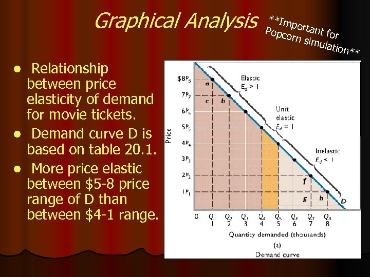Graphical Analysis Relationship between price elasticity of demand for movie tickets. l Demand curve D is based on table 20. 1. l More price elastic between $5 -8 price range of D than between $4 -1 range. l **Im p Popc ortant for orn s imula tion* *

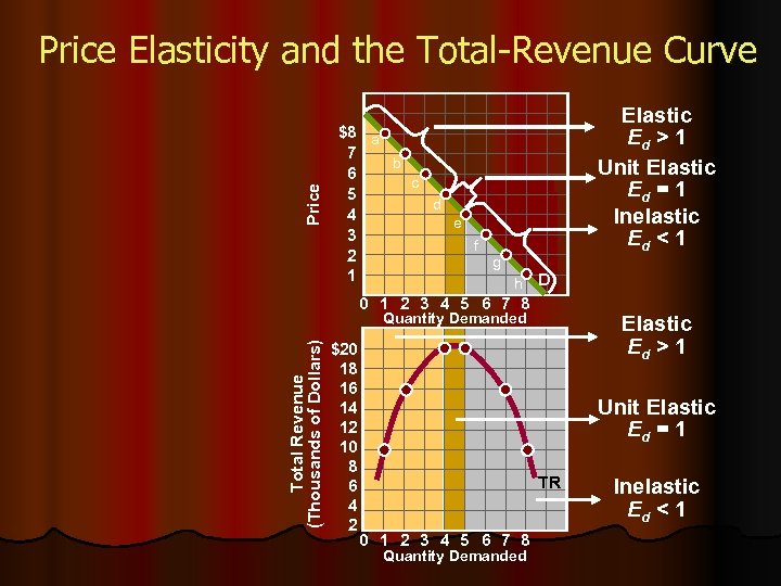Price Elasticity and the Total-Revenue Curve $8 a 7 b 6 c 5 d 4 e 3 f 2 g 1 h D 0 1 2 3 4 5 6 7 8 Total Revenue (Thousands of Dollars) Quantity Demanded $20 18 16 14 12 10 8 6 4 2 Elastic Ed > 1 Unit Elastic Ed = 1 Inelastic Ed < 1 Elastic Ed > 1 Unit Elastic Ed = 1 TR 0 1 2 3 4 5 6 7 8 Quantity Demanded Inelastic Ed < 1

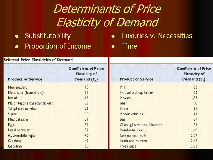Determinants of Price Elasticity of Demand Substitutability l Proportion of Income l ● Luxuries v. Necessities ● Time

Applications of Price Elasticity of Demand Large crop yields Typical examples of excise duties are taxes on gasoline, l Excise tax tobacco and alcohol (sometimes referred to as sin taxes). l Decriminalize illegal drugs l Minimum wage ($8/CA, $7. 25/Fed) l

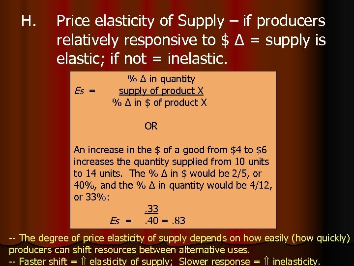H. Price elasticity of Supply – if producers relatively responsive to $ Δ = supply is elastic; if not = inelastic. Es = % Δ in quantity supply of product X % Δ in $ of product X OR An increase in the $ of a good from $4 to $6 increases the quantity supplied from 10 units to 14 units. The % Δ in $ would be 2/5, or 40%, and the % Δ in quantity would be 4/12, or 33%: . 33 Es =. 40 =. 83 -- The degree of price elasticity of supply depends on how easily (how quickly) producers can shift resources between alternative uses. -- Faster shift = elasticity of supply; Slower response = inelasticity.

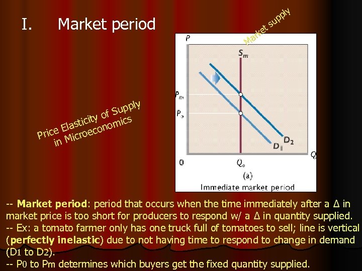I. Market period t ke r Ma ly pp su ly p Sup f ity o mics tic Elas econo Price Micro in -- Market period: period that occurs when the time immediately after a Δ in market price is too short for producers to respond w/ a Δ in quantity supplied. -- Ex: a tomato farmer only has one truck full of tomatoes to sell; line is vertical (perfectly inelastic) due to not having time to respond to change in demand (D 1 to D 2). -- P 0 to Pm determines which buyers get the fixed quantity supplied.

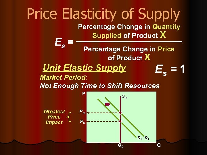Price Elasticity of Supply Es = Percentage Change in Quantity Supplied of Product X Percentage Change in Price of Product X Unit Elastic Supply Es = 1 Market Period: Not Enough Time to Shift Resources P Greatest Price Impact Sm Pm P 0 D 1 D 2 Q 0 Q

1. 2. Short run Long run Price E lasticit y of Su in Micr pply oecon omics -- Short run – period of time too short to change plant capacity but long enough to use fixed plant more or less inexpensively (fixed land/farm machinery, but can use more labor/fertilizer) for more output (more elastic). -- Long run – time period long enough for firms to adjust their plant sizes & for new firms to enter (or existing to leave) the industry (still more elastic). -- There is no total-revenue test for elasticity of supply. -- Supply shows a positive (direct relationship) between $ & amount supplied.

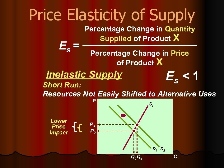Price Elasticity of Supply Es = Percentage Change in Quantity Supplied of Product X Percentage Change in Price of Product X Inelastic Supply Es < 1 Short Run: Resources Not Easily Shifted to Alternative Uses P Lower Price Impact Ss Ps P 0 D 1 D 2 Q 0 Qs Q

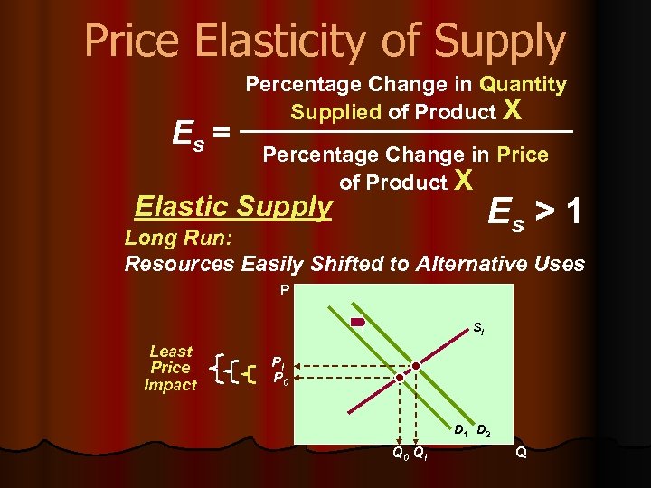Price Elasticity of Supply Es = Percentage Change in Quantity Supplied of Product X Percentage Change in Price of Product X Elastic Supply Es > 1 Long Run: Resources Easily Shifted to Alternative Uses P Sl Least Price Impact Pl P 0 D 1 D 2 Q 0 Ql Q

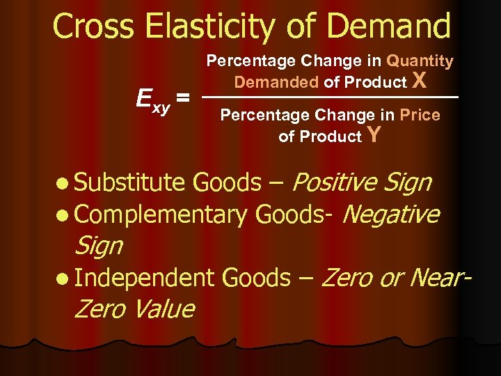
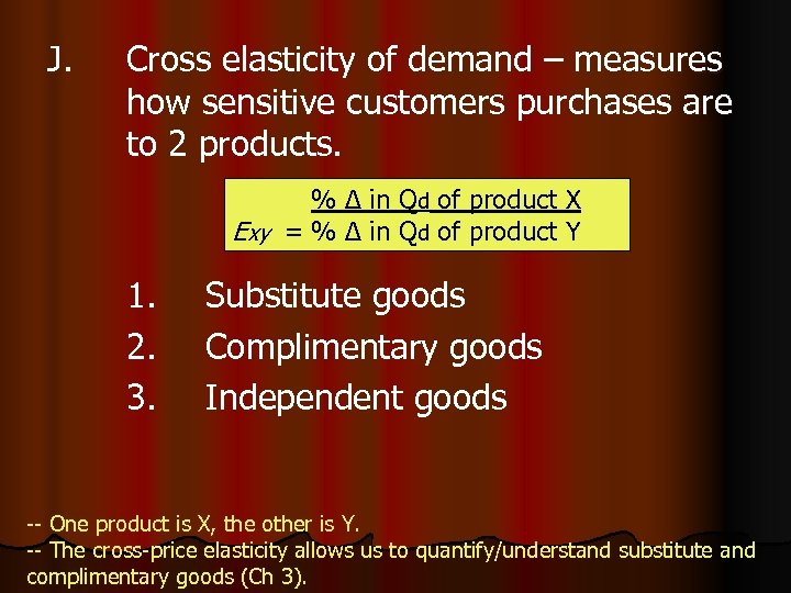J. Cross elasticity of demand – measures how sensitive customers purchases are to 2 products. % Δ in Qd of product X Exy = % Δ in Qd of product Y 1. 2. 3. Substitute goods Complimentary goods Independent goods -- One product is X, the other is Y. -- The cross-price elasticity allows us to quantify/understand substitute and complimentary goods (Ch 3).

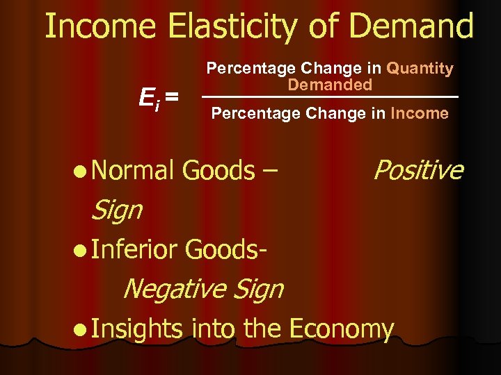
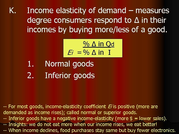K. Income elasticity of demand – measures degree consumers respond to Δ in their incomes by buying more/less of a good. % Δ in Qd Ei = % Δ in I 1. 2. Normal goods Inferior goods -- For most goods, income-elasticity coefficient Ei is positive (more are demanded as income rises); called normal or superior goods. -- Inferior goods have a negative income-elasticity (more $ = lower sales). -- Insights: we do not eat more when our income rises, we eat better! -- When income declines, food purchases stay same but buy fewer electronics.

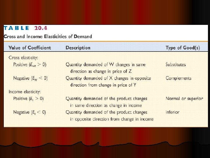
Cross Elasticity of Demand Exy = Percentage Change in Quantity Demanded of Product X Percentage Change in Price of Product Y Goods – Positive Sign l Complementary Goods- Negative l Substitute Sign l Independent Zero Value Goods – Zero or Near-

Income Elasticity of Demand Percentage Change in Quantity Demanded Ei = l Normal Percentage Change in Income Goods – Positive Sign l Inferior Goods- Negative Sign l Insights into the Economy

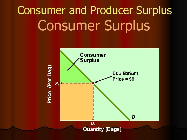Consumer and Producer Surplus Consumer Surplus Price (Per Bag) Consumer Surplus Equilibrium Price = $8 P 1 D Q 1 Quantity (Bags)

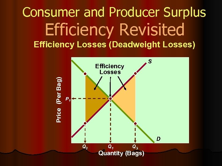Consumer and Producer Surplus Efficiency Revisited Efficiency Losses (Deadweight Losses) S Price (Per Bag) Efficiency Losses P 1 D Q 2 Q 1 Q 3 Quantity (Bags)