CERN Genève 18 December 2013 Scientific collaboration with

CERN Genève 18 December 2013 Scientific collaboration with CERN F. Assous J. Chaskalovic Mathematics Department Institut Jean le Rond d’Alembert Bar Ilan Ariel University Pierre and Marie Curie

Agenda The team Theoretical and numerical approaches for charged particle beams Actual items Our future projects Data Mining for the CERN

The team

The team Franck Assous: Academic and industrial experiment Ph. D in Applied Mathematics (Dauphine University, Paris 9). Associate Professor in Applied Mathematics, Bar Ilan Ariel University, (Israel). Scientific Consultant, CEA, (France), (1990 -2002). Joel Chaskalovic: Dual expertise Ph. D in Theoretical Mechanics (University Pierre & Marie Curie) and Engineer of « Ecole Nationale des Ponts & Chaussées » . Associate Professor in Mathematical Modeling applied to Engineering Sciences, (University Pierre & Marie Curie). Director of Data Mining and Media Research, Publicis Group, (1993 -2007).

Theoretical and numerical approaches for particles accelerators

Actual items A new method to evaluate asymptotic numerical models by Data Mining techniques On a new paraxial model Data Mining: a tool to evaluate the quality of models

A new method to evaluate asymptotic numerical models by Data Mining techniques

The physical problem • Physical frameworks: collisionless charged particles beams (Accelerators, F. E. L, …)

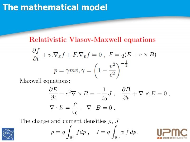
The mathematical model

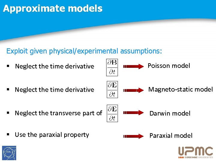
Approximate models Exploit given physical/experimental assumptions: § Neglect the time derivative Poisson model § Neglect the time derivative Magneto-static model § Neglect the transverse part of Darwin model § Use the paraxial property Paraxial model

How we derive a paraxial model 1. Write the equations in the beam frame. 2. Introduce a scaling of the equations. 3. Define a small parameter. 4. Use expansion techniques and retains the first orders. 5. Build an ad hoc discretization. 6. Simulations with numerical results.

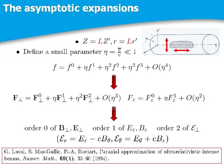
The asymptotic expansions

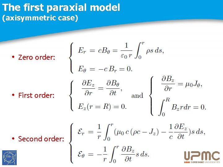
The first paraxial model (axisymmetric case) • Zero order: • First order: • Second order:

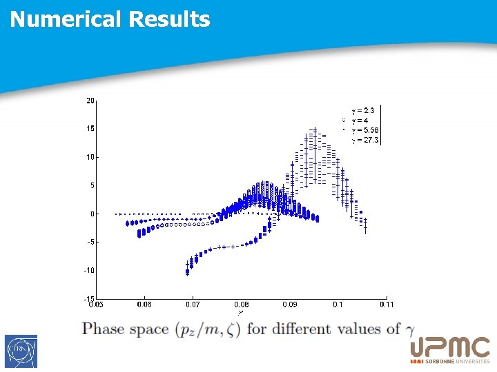
Numerical Results

But…fundamental questions Despite a theoretical result (controlled accuracy)… How many terms to retain in the asymptotic expansion to get a “precise” model ? How to compare the different orders of approximation: - What each order of the asymptotic expansion brings to the numerical results ? - Which variables are responsible of the improvement between models Mi and Mi+1 ? Use of Data Mining Methodology

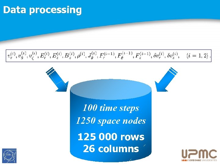
Data processing 100 time steps 1250 space nodes 125 000 rows 26 columns

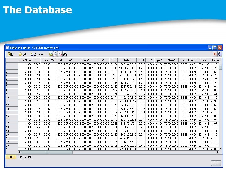
The Database

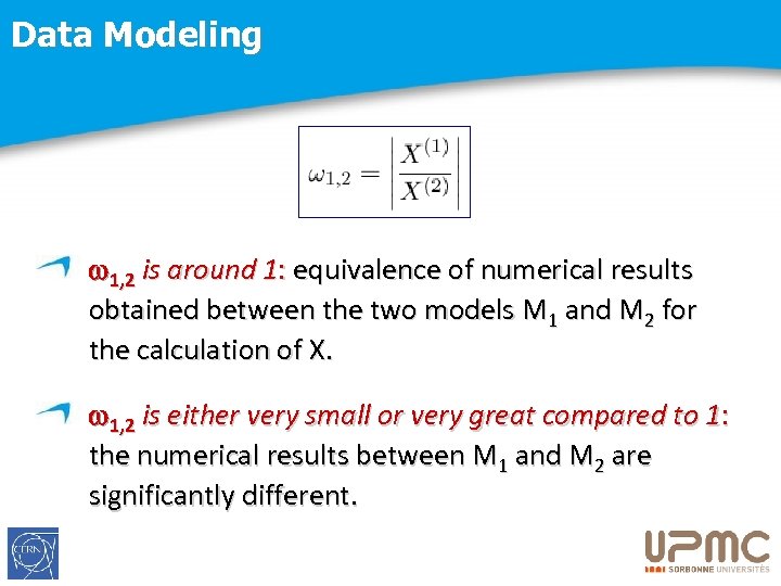
Data Modeling 1, 2 is around 1: equivalence of numerical results obtained between the two models M 1 and M 2 for the calculation of X. 1, 2 is either very small or very great compared to 1: the numerical results between M 1 and M 2 are significantly different.

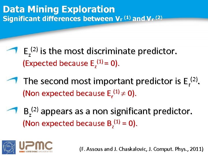
Data Mining Exploration Significant differences between Vr (1) and Vr (2) Ez(2) is the most discriminate predictor. (Expected because Ez(1) = 0). The second most important predictor is Er(2). (Non expected because Er(1) 0). Bz(2) appears as a non significant predictor. (Non expected because Bz(1) = 0). (F. Assous and J. Chaskalovic, J. Comput. Phys. , 2011)

Future developments Which is the best asymptotic expansion? Globally the second order is better than the first order. But locally, could we status when and where the first one could be better ? Data Experiments and Data Mining

On a new paraxial model

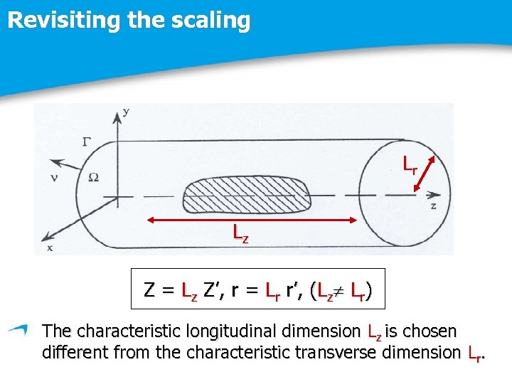
Revisiting the scaling Lr Lz Z = Lz Z’, r = Lr r’, (Lz Lr) The characteristic longitudinal dimension Lz is chosen different from the characteristic transverse dimension Lr.

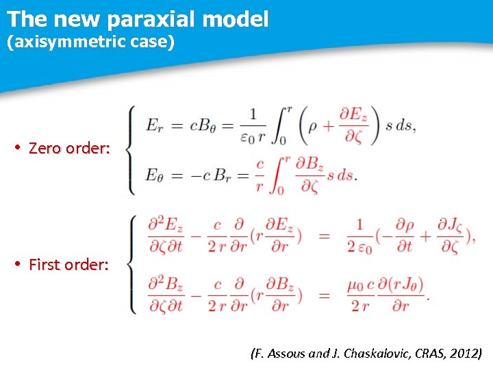
The new paraxial model (axisymmetric case) • Zero order: • First order: (F. Assous and J. Chaskalovic, CRAS, 2012)

Future developments Numerical simulations. Validation and characterization by Data Mining techniques of significant differences between the two asymptotic models (Lz = Lr) and (Lz Lr). Comparison with experimental data.

Data Mining a tool to evaluate the quality of models

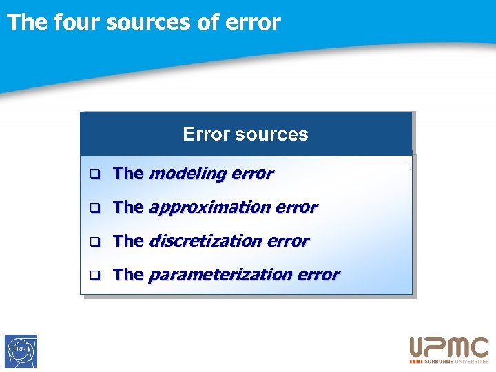
The four sources of error Error sources q The modeling error q The approximation error q The discretization error q The parameterization error

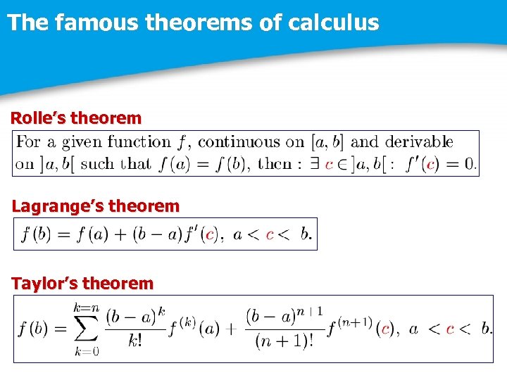
The famous theorems of calculus Rolle’s theorem Lagrange’s theorem Taylor’s theorem

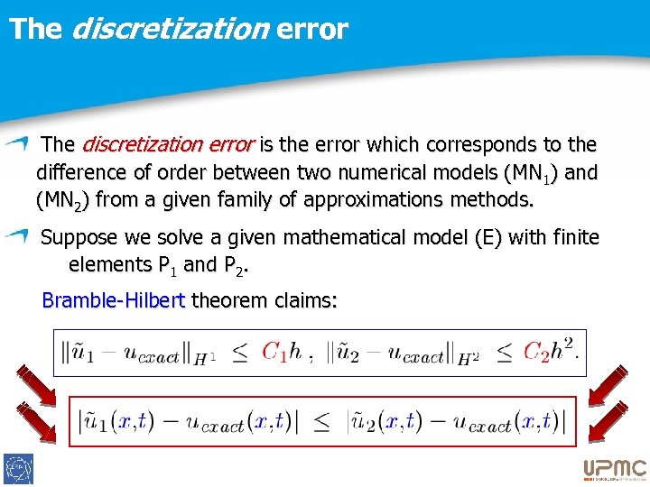
The discretization error is the error which corresponds to the difference of order between two numerical models (MN 1) and (MN 2) from a given family of approximations methods. Suppose we solve a given mathematical model (E) with finite elements P 1 and P 2. Bramble-Hilbert theorem claims:

The discretization error P 1 - P 2 finite elements method for numerical approximation to Vlasov-Maxwell equations

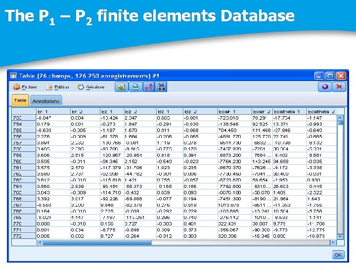
The P 1 – P 2 finite elements Database

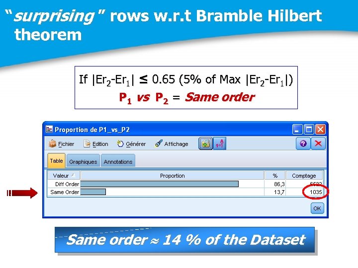
“surprising ” rows w. r. t Bramble Hilbert theorem If |Er 2 -Er 1| ≤ 0. 65 (5% of Max |Er 2 -Er 1|) P 1 vs P 2 = Same order 14 % of the Dataset

Kohonen’ cards

Kohonen’s Cluster Analysis

Rules of Cluster “P 1 – P 2 same order” P 1 vs P 2

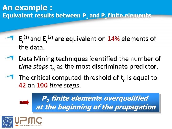
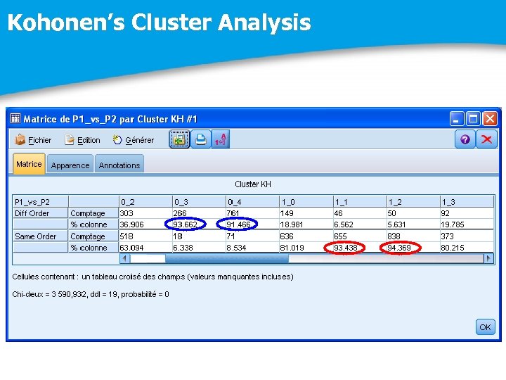
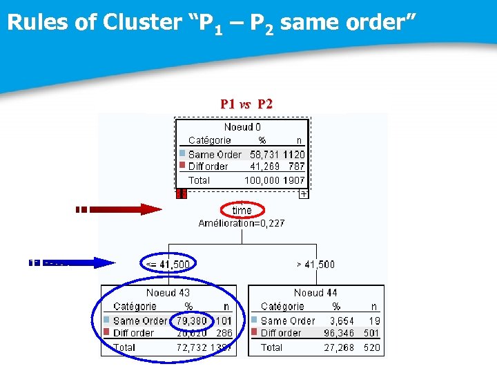
An example : Equivalent results between P 1 and P 2 finite elements Er(1) and Er(2) are equivalent on 14% elements of the data. Data Mining techniques identified the number of time steps tn as the most discriminate predictor. The critical computed threshold of tn is equal to 42 on 100 time steps. P 2 finite elements overqualified at the beginning of the propagation

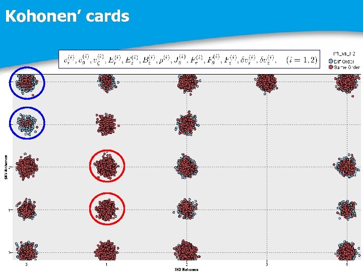
Future developments Physical interpretations of the above results : The threshold tn = 42. Robustness of the results: comparison with other data technologies, (Neural Networks, Kohonen Cards, etc. ). Extensions to other physical unknowns. Sensibility regarding the Data. Coupling errors. Data Mining

Data Mining for the CERN

The CERN and the Data Mining « Les expériences du Large Hadron Collider représentent environ 150 millions de capteurs délivrant des données 40 millions de fois par seconde. Il y a autour de 600 millions de collisions par seconde, et après filtrage, il reste 100 collisions d’intérêt par seconde. En conséquence, il y a 25 Po de données à stocker chaque année. » (source : Wikipédia)

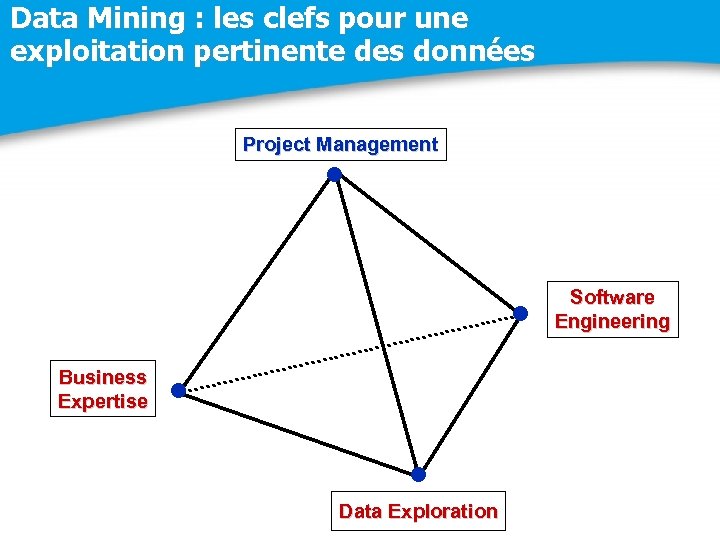
Data Mining : les clefs pour une exploitation pertinente des données Project Management • • Business Expertise • • Data Exploration Software Engineering

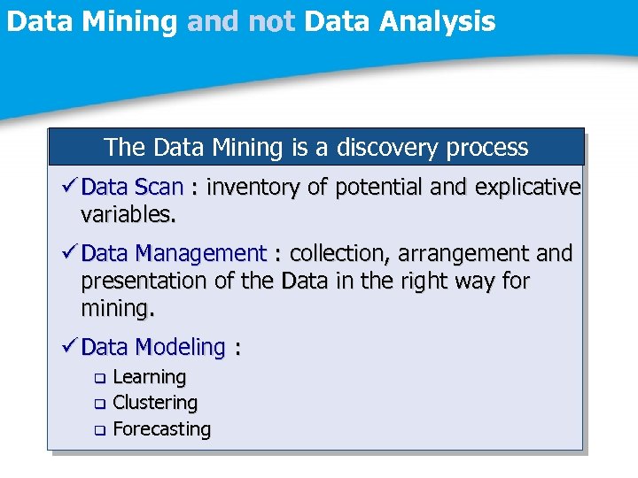
Data Mining and not Data Analysis The Data Mining is a discovery process ü Data Scan : inventory of potential and explicative variables. ü Data Management : collection, arrangement and presentation of the Data in the right way for mining. ü Data Modeling : Learning q Clustering q Forecasting q

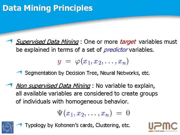
Data Mining Principles Supervised Data Mining : One or more target variables must be explained in terms of a set of predictor variables. Segmentation by Decision Tree, Neural Networks, etc. Non supervised Data Mining : No variable to explain, all available variables are considered to create groups of individuals with homogeneous behavior. Typology by Kohonen’s cards, Clustering, etc.

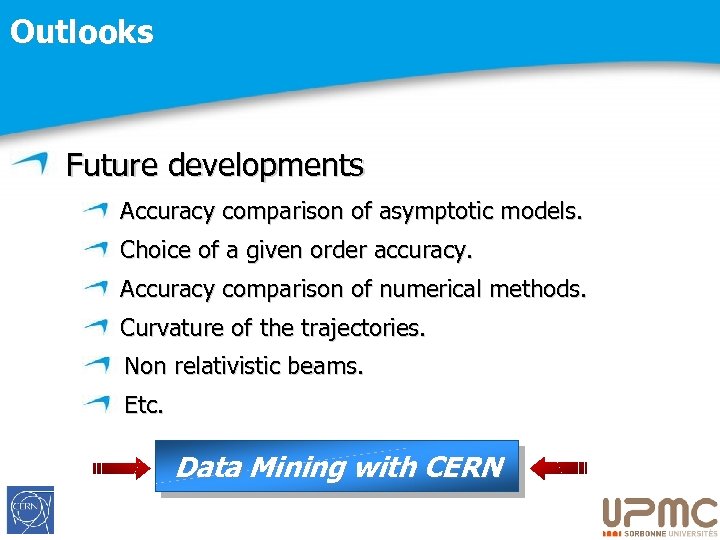
Outlooks Future developments Accuracy comparison of asymptotic models. Choice of a given order accuracy. Accuracy comparison of numerical methods. Curvature of the trajectories. Non relativistic beams. Etc. Data Mining with CERN

Merci !