63b201a5d455b69427eac40c4cecead1.ppt
- Количество слайдов: 83
 CAUSAL INFERENCE IN STATISTICS A Gentle Introduction Judea Pearl University of California Los Angeles (www. cs. ucla. edu/~judea/jsm 09)
 OUTLINE • Inference: Statistical vs. Causal, distinctions, and mental barriers • Unified conceptualization of counterfactuals, structural-equations, and graphs • Inference to three types of claims: 1. Causal effects and confounding 2. Attribution (Causes of Effects) 3. Direct and indirect effects • Frills – external validity and transportability
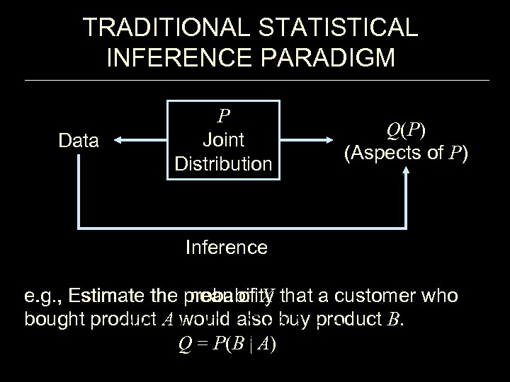 TRADITIONAL STATISTICAL INFERENCE PARADIGM Data P Joint Distribution Q(P) (Aspects of P) Inference e. g. , Estimate the mean of X e. g. , Estimate the probability that a customer who bought product A would also buy product B. Q = P(B | A)
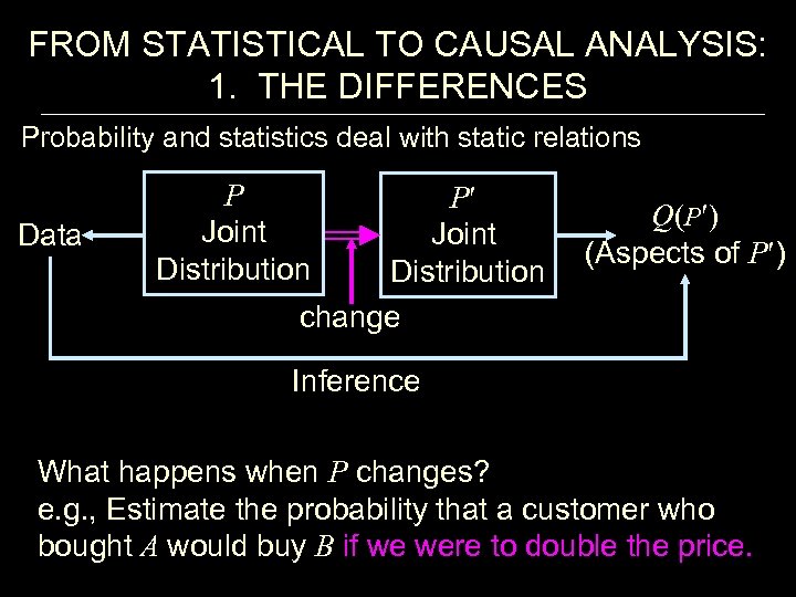 FROM STATISTICAL TO CAUSAL ANALYSIS: 1. THE DIFFERENCES Probability and statistics deal with static relations Data P Joint Distribution P Joint Distribution change Q(P ) (Aspects of P ) Inference What happens when P changes? e. g. , Estimate the probability that a customer who bought A would buy B if we were to double the price.
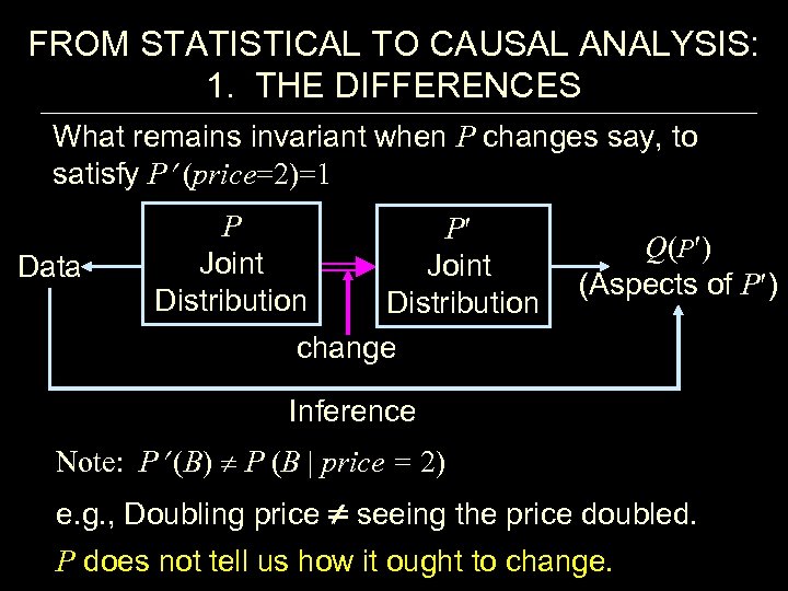 FROM STATISTICAL TO CAUSAL ANALYSIS: 1. THE DIFFERENCES What remains invariant when P changes say, to satisfy P (price=2)=1 Data P Joint Distribution P Joint Distribution change Q(P ) (Aspects of P ) Inference Note: P (B) P (B | price = 2) e. g. , Doubling price seeing the price doubled. P does not tell us how it ought to change.
 FROM STATISTICAL TO CAUSAL ANALYSIS: 1. THE DIFFERENCES (CONT) 1. Causal and statistical concepts do not mix. CAUSAL Spurious correlation Randomization / Intervention Confounding / Effect Instrumental variable Ignorability / Exogeneity Explanatory variables 2. 3. 4. STATISTICAL Regression Association / Independence “Controlling for” / Conditioning Odd and risk ratios Collapsibility / Granger causality Propensity score

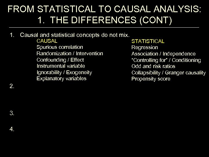 FROM STATISTICAL TO CAUSAL ANALYSIS: 1. THE DIFFERENCES (CONT) 1. Causal and statistical concepts do not mix. CAUSAL Spurious correlation Randomization / Intervention Confounding / Effect Instrumental variable Ignorability / Exogeneity Explanatory variables 2. 3. 4. STATISTICAL Regression Association / Independence “Controlling for” / Conditioning Odd and risk ratios Collapsibility / Granger causality Propensity score
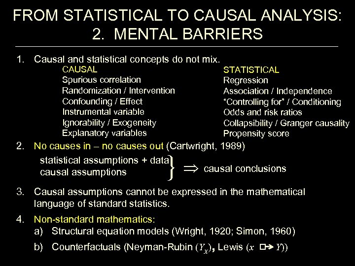 FROM STATISTICAL TO CAUSAL ANALYSIS: 2. MENTAL BARRIERS 1. Causal and statistical concepts do not mix. CAUSAL Spurious correlation Randomization / Intervention Confounding / Effect Instrumental variable Ignorability / Exogeneity Explanatory variables STATISTICAL Regression Association / Independence “Controlling for” / Conditioning Odds and risk ratios Collapsibility / Granger causality Propensity score 2. No causes in – no causes out (Cartwright, 1989) statistical assumptions + data causal conclusions causal assumptions } 3. Causal assumptions cannot be expressed in the mathematical language of standard statistics. 4. Non-standard mathematics: a) Structural equation models (Wright, 1920; Simon, 1960) b) Counterfactuals (Neyman-Rubin (Yx), Lewis (x Y))
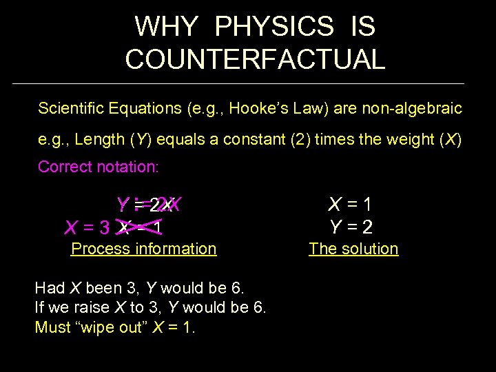 WHY PHYSICS IS COUNTERFACTUAL Scientific Equations (e. g. , Hooke’s Law) are non-algebraic e. g. , Length (Y) equals a constant (2) times the weight (X) Correct notation: Y : =2 X = 2 X X=3 X=1 Process information Had X been 3, Y would be 6. If we raise X to 3, Y would be 6. Must “wipe out” X = 1. X=1 Y=2 The solution
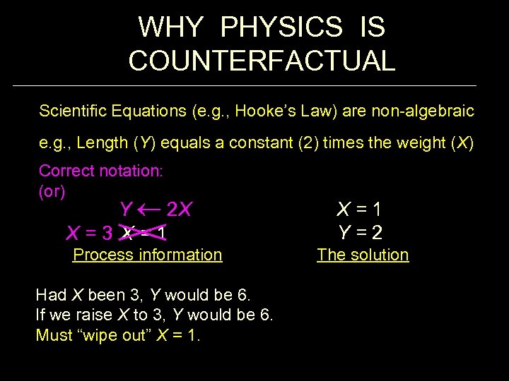 WHY PHYSICS IS COUNTERFACTUAL Scientific Equations (e. g. , Hooke’s Law) are non-algebraic e. g. , Length (Y) equals a constant (2) times the weight (X) Correct notation: (or) Y 2 X X=3 X=1 Process information Had X been 3, Y would be 6. If we raise X to 3, Y would be 6. Must “wipe out” X = 1. X=1 Y=2 The solution
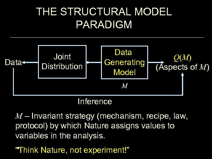 THE STRUCTURAL MODEL PARADIGM Data Joint Distribution Data Generating Model Q(M) (Aspects of M) M Inference M – Invariant strategy (mechanism, recipe, law, protocol) by which Nature assigns values to variables in the analysis. • “Think Nature, not experiment!”
 FAMILIAR CAUSAL MODEL ORACLE FOR MANIPILATION X Y Z INPUT OUTPUT
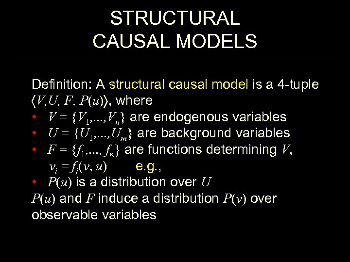 STRUCTURAL CAUSAL MODELS Definition: A structural causal model is a 4 -tuple V, U, F, P(u) , where • V = {V 1, . . . , Vn} are endogenous variables • U = {U 1, . . . , Um} are background variables • F = {f 1, . . . , fn} are functions determining V, vi = fi(v, u) e. g. , • P(u) is a distribution over U P(u) and F induce a distribution P(v) over observable variables
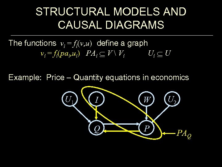 STRUCTURAL MODELS AND CAUSAL DIAGRAMS The functions vi = fi(v, u) define a graph vi = fi(pai, ui) PAi V Vi Ui U Example: Price – Quantity equations in economics U 1 I W Q P U 2 PAQ
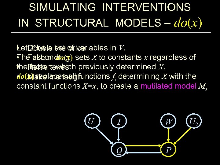 SIMULATING INTERVENTIONS IN STRUCTURAL MODELS – do(x) Let X be a set of variables in V. • Double the price The action do(x) sets X to constants x regardless of • Take a drug the factors which previously determined X. • Raise taxes do(x) replaces all functions fi determining X with the • Make me laugh constant functions X=x, to create a mutilated model Mx U 1 I W Q P U 2
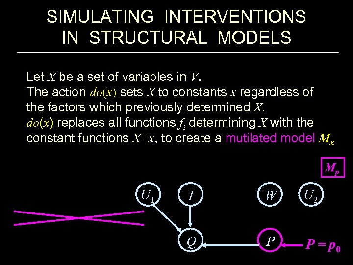 SIMULATING INTERVENTIONS IN STRUCTURAL MODELS Let X be a set of variables in V. The action do(x) sets X to constants x regardless of the factors which previously determined X. do(x) replaces all functions fi determining X with the constant functions X=x, to create a mutilated model Mx Mp U 1 I W U 2 Q P P = p 0
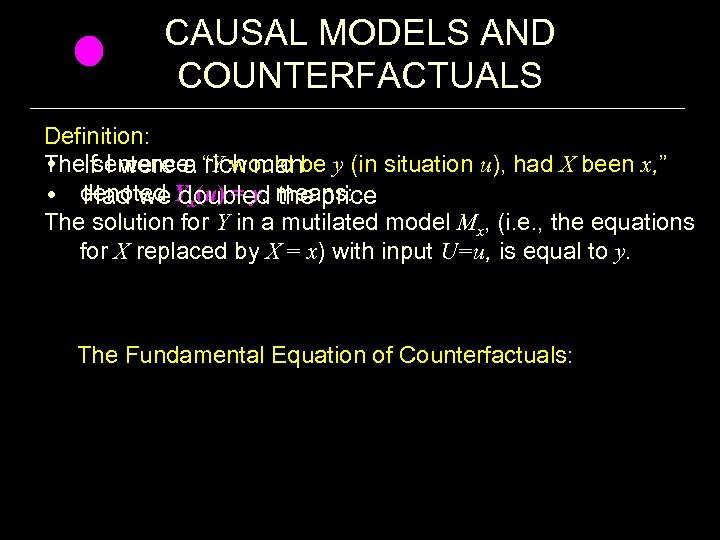 CAUSAL MODELS AND COUNTERFACTUALS Definition: The sentence: “Y would be y (in situation u), had X been x, ” • If I were a rich man • denoted Yx(u) = y, means: Had we doubled the price The solution for Y in a mutilated model Mx, (i. e. , the equations for X replaced by X = x) with input U=u, is equal to y. The Fundamental Equation of Counterfactuals:
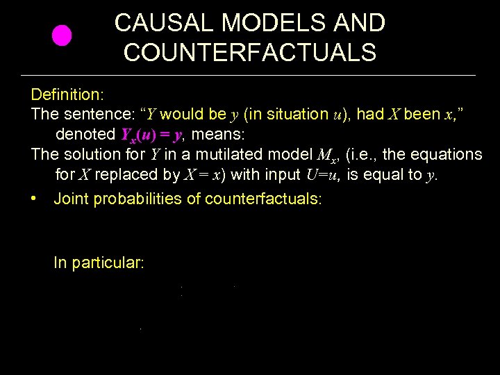 CAUSAL MODELS AND COUNTERFACTUALS Definition: The sentence: “Y would be y (in situation u), had X been x, ” denoted Yx(u) = y, means: The solution for Y in a mutilated model Mx, (i. e. , the equations for X replaced by X = x) with input U=u, is equal to y. • Joint probabilities of counterfactuals: In particular:
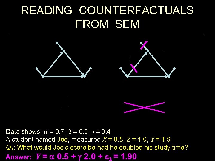 READING COUNTERFACTUALS FROM SEM Data shows: a = 0. 7, b = 0. 5, g = 0. 4 A student named Joe, measured X = 0. 5, Z = 1. 0, Y = 1. 9 Q 1: What would Joe’s score be had he doubled his study time? Answer: Y = 0. 5 + 2. 0 + = 1. 90
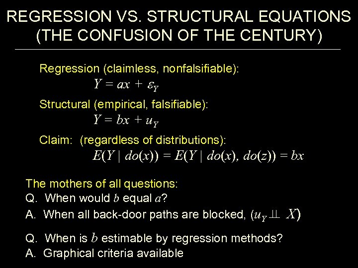 REGRESSION VS. STRUCTURAL EQUATIONS (THE CONFUSION OF THE CENTURY) Regression (claimless, nonfalsifiable): Y = ax + Y Structural (empirical, falsifiable): Y = bx + u. Y Claim: (regardless of distributions): E(Y | do(x)) = E(Y | do(x), do(z)) = bx The mothers of all questions: Q. When would b equal a? A. When all back-door paths are blocked, (u. Y X) Q. When is b estimable by regression methods? A. Graphical criteria available
 THE FIVE NECESSARY STEPS OF CAUSAL ANALYSIS Define: Express the target quantity Q as property of the model M. Assume: Express causal assumptions in structural or graphical form. Identify: Determine if Q is identifiable. Estimate: Estimate Q if it is identifiable; approximate it, if it is not. Test: If M has testable implications Repeat if necessary
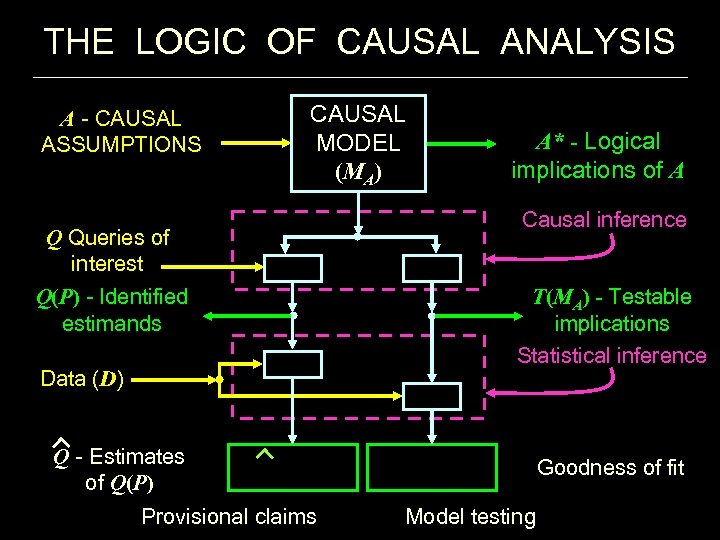 THE LOGIC OF CAUSAL ANALYSIS A - CAUSAL ASSUMPTIONS CAUSAL MODEL (MA) Q Queries of interest Q(P) - Identified estimands Data (D) A* - Logical implications of A Causal inference T(MA) - Testable implications Statistical inference Q - Estimates of Q(P) Provisional claims Goodness of fit Model testing
 THE FIVE NECESSARY STEPS FOR EFFECT ESTIMATION Define: Express the target quantity Q as a property of the model M. Assume: Express causal assumptions in structural or graphical form. Identify: Determine if Q is identifiable. Estimate: Estimate Q if it is identifiable; approximate it, if it is not. Test: If M has testable implications
 THE FIVE NECESSARY STEPS FOR AVERAGE TREATMENT EFFECT Define: Express the target quantity Q as a property of the model M. Assume: Express causal assumptions in structural or graphical form. Identify: Determine if Q is identifiable. Estimate: Estimate Q if it is identifiable; approximate it, if it is not. Test: If M has testable implications
 THE FIVE NECESSARY STEPS FOR DYNAMIC POLICY ANALYSIS Define: Express the target quantity Q as a property of the model M. Assume: Express causal assumptions in structural or graphical form. Identify: Determine if Q is identifiable. Estimate: Estimate Q if it is identifiable; approximate it, if it is not. Test: If M has testable implications
 THE FIVE NECESSARY STEPS FOR TIME VARYING POLICY ANALYSIS Define: Express the target quantity Q as a property of the model M. Assume: Express causal assumptions in structural or graphical form. Identify: Determine if Q is identifiable. Estimate: Estimate Q if it is identifiable; approximate it, if it is not. Test: If M has testable implications
 THE FIVE NECESSARY STEPS FOR TREATMENT ON TREATED Define: Express the target quantity Q a property of the model M. Assume: Express causal assumptions in structural or graphical form. Identify: Determine if Q is identifiable. Estimate: Estimate Q if it is identifiable; approximate it, if it is not. Test: If M has testable implications
 THE FIVE NECESSARY STEPS FOR INDIRECT EFFECTS Define: Express the target quantity Q a property of the model M. Assume: Express causal assumptions in structural or graphical form. Identify: Determine if Q is identifiable. Estimate: Estimate Q if it is identifiable; approximate it, if it is not. Test: If M has testable implications
 THE FIVE NECESSARY STEPS FROM DEFINITION TO ASSUMPTIONS Define: Express the target quantity Q as a property of the model M. Assume: Express causal assumptions in structural or graphical form. Identify: Determine if Q is identifiable. Estimate: Estimate Q if it is identifiable; approximate it, if it is not. Test: If M has testable implications
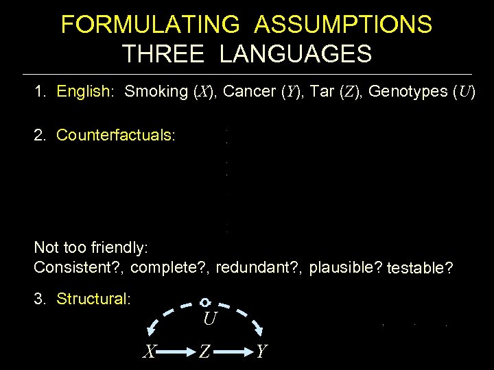 FORMULATING ASSUMPTIONS THREE LANGUAGES 1. English: Smoking (X), Cancer (Y), Tar (Z), Genotypes (U) 2. Counterfactuals: Not too friendly: Consistent? , complete? , redundant? , plausible? testable? 3. Structural: U X Z Y
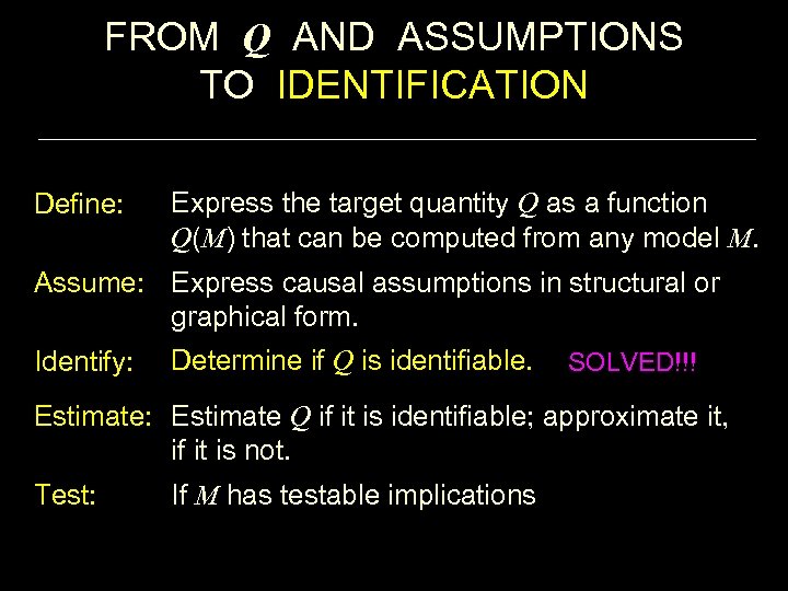 FROM Q AND ASSUMPTIONS TO IDENTIFICATION Define: Express the target quantity Q as a function Q(M) that can be computed from any model M. Assume: Express causal assumptions in structural or graphical form. Identify: Determine if Q is identifiable. SOLVED!!! Estimate: Estimate Q if it is identifiable; approximate it, if it is not. Test: If M has testable implications
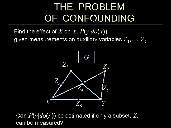 THE PROBLEM OF CONFOUNDING Find the effect of X on Y, P(y|do(x)), given measurements on auxiliary variables Z 1, . . . , Zk G Z 1 Z 3 X Z 2 Z 4 Z 5 Z 6 Y Can P(y|do(x)) be estimated if only a subset, Z, can be measured?
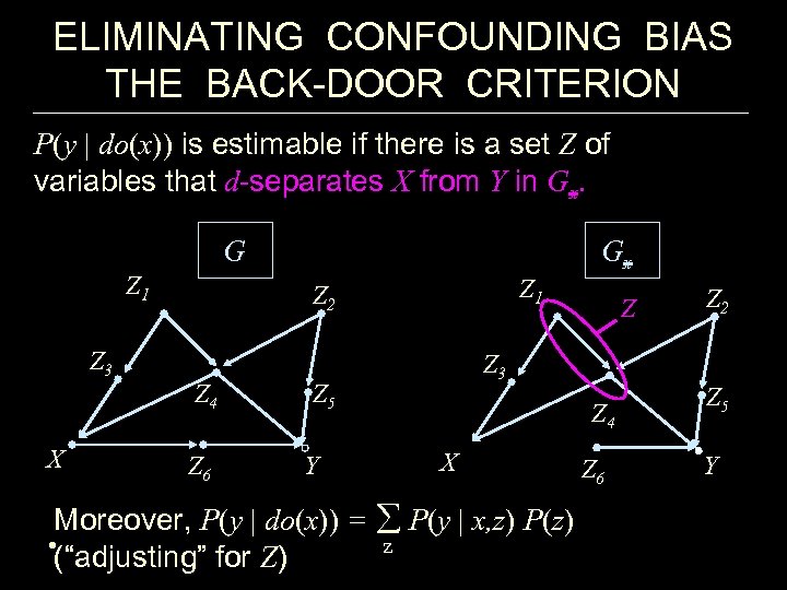 ELIMINATING CONFOUNDING BIAS THE BACK-DOOR CRITERION P(y | do(x)) is estimable if there is a set Z of variables that d-separates X from Y in Gx. G Z 1 Z 3 X Gx Z 1 Z 2 Z 4 Z 6 Z 3 Z 5 Y Z Z 4 X Moreover, P(y | do(x)) = å P(y | x, z) P(z) z • (“adjusting” for Z) Z 6 Z 2 Z 5 Y
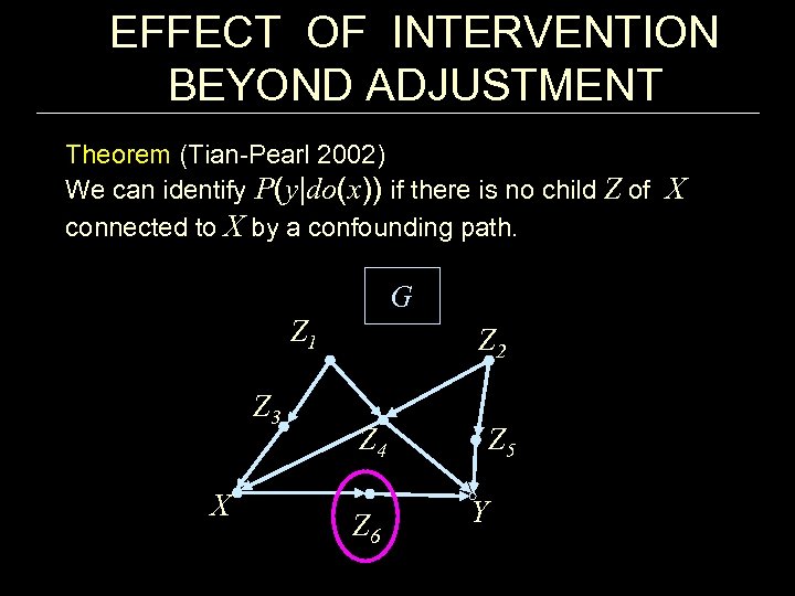 EFFECT OF INTERVENTION BEYOND ADJUSTMENT Theorem (Tian-Pearl 2002) We can identify P(y|do(x)) if there is no child Z of X connected to X by a confounding path. G Z 1 Z 3 X Z 2 Z 4 Z 6 Z 5 Y
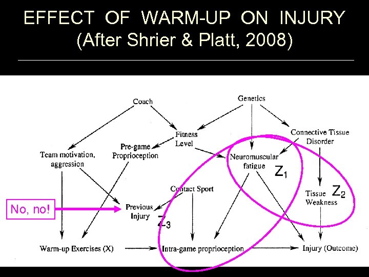 EFFECT OF WARM-UP ON INJURY (After Shrier & Platt, 2008) No, no!
 COUNTERFACTUALS AT WORK ETT – EFFECT OF TREATMENT ON THE TREATED 1. Regret: I took a pill to fall asleep. Perhaps I should not have? 2. Program evaluation: What would terminating a program do to those enrolled?
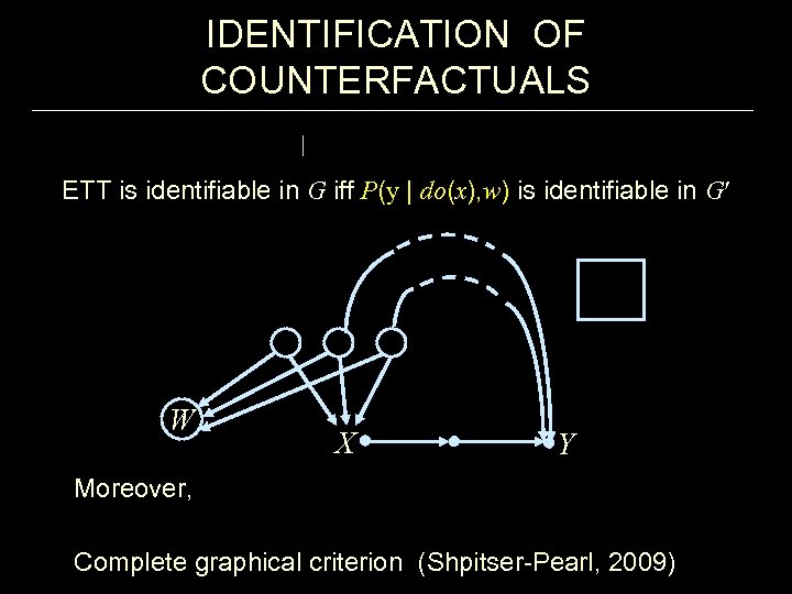 IDENTIFICATION OF COUNTERFACTUALS ETT is identifiable in G iff P(y | do(x), w) is identifiable in G W X Y Moreover, Complete graphical criterion (Shpitser-Pearl, 2009)
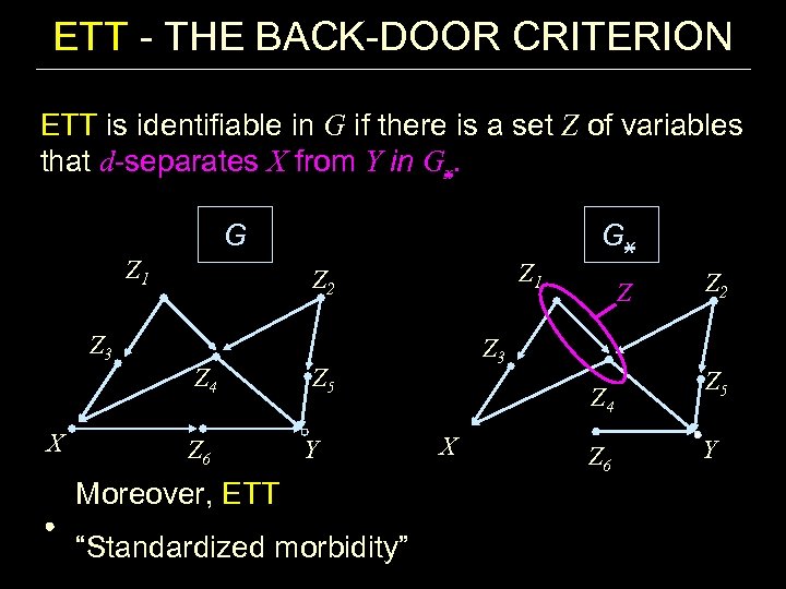 ETT - THE BACK-DOOR CRITERION ETT is identifiable in G if there is a set Z of variables that d-separates X from Y in Gx. G Z 1 Z 3 X Gx Z 1 Z 2 Z 4 Z 6 Z 3 Z 5 Y Moreover, ETT “Standardized morbidity” Z Z 4 X Z 6 Z 2 Z 5 Y
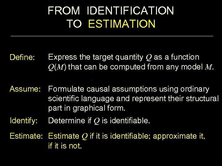 FROM IDENTIFICATION TO ESTIMATION Define: Express the target quantity Q as a function Q(M) that can be computed from any model M. Assume: Formulate causal assumptions using ordinary scientific language and represent their structural part in graphical form. Identify: Determine if Q is identifiable. Estimate: Estimate Q if it is identifiable; approximate it, if it is not.
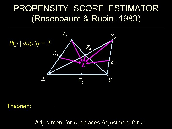 PROPENSITY SCORE ESTIMATOR (Rosenbaum & Rubin, 1983) Z 1 Z 2 P(y | do(x)) = ? Z 4 Z 3 L X Z 6 Z 5 Y Theorem: Adjustment for L replaces Adjustment for Z
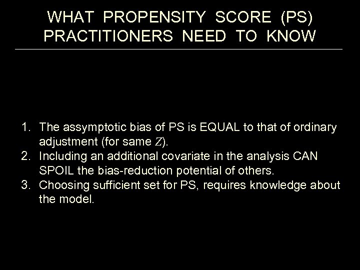 WHAT PROPENSITY SCORE (PS) PRACTITIONERS NEED TO KNOW 1. The assymptotic bias of PS is EQUAL to that of ordinary adjustment (for same Z). 2. Including an additional covariate in the analysis CAN SPOIL the bias-reduction potential of others. 3. Choosing sufficient set for PS, requires knowledge about the model.
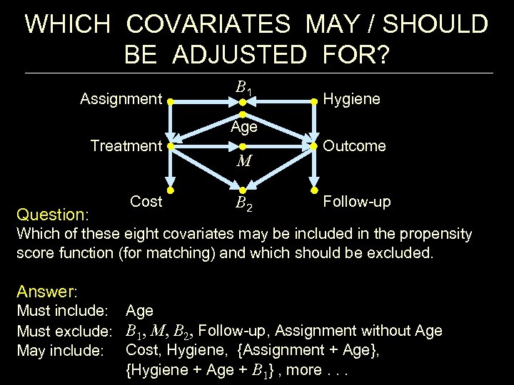 WHICH COVARIATES MAY / SHOULD BE ADJUSTED FOR? Assignment B 1 Hygiene Age Treatment Question: Cost M B 2 Outcome Follow-up Which of these eight covariates may be included in the propensity score function (for matching) and which should be excluded. Answer: Age Must include: Must exclude: B 1, M, B 2, Follow-up, Assignment without Age Cost, Hygiene, {Assignment + Age}, May include: {Hygiene + Age + B 1} , more. . .
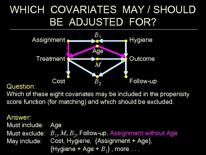 WHICH COVARIATES MAY / SHOULD BE ADJUSTED FOR? Assignment B 1 Hygiene Age Treatment Question: Cost M B 2 Outcome Follow-up Which of these eight covariates may be included in the propensity score function (for matching) and which should be excluded. Answer: Age Must include: Must exclude: B 1, M, B 2, Follow-up, Assignment without Age Cost, Hygiene, {Assignment + Age}, May include: {Hygiene + Age + B 1} , more. . .
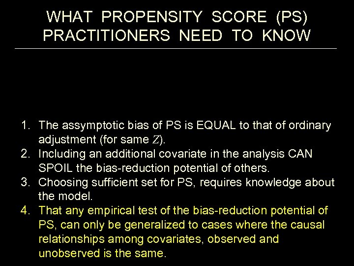 WHAT PROPENSITY SCORE (PS) PRACTITIONERS NEED TO KNOW 1. The assymptotic bias of PS is EQUAL to that of ordinary adjustment (for same Z). 2. Including an additional covariate in the analysis CAN SPOIL the bias-reduction potential of others. 3. Choosing sufficient set for PS, requires knowledge about the model. 4. That any empirical test of the bias-reduction potential of PS, can only be generalized to cases where the causal relationships among covariates, observed and unobserved is the same.
 THE STRUCTURAL-COUNTERFACTUAL SYMBIOSIS 1. Express assumptions in structural or graphical language. 2. Express queries in counterfactual language. 3. 3. Translate (1) into (2) for algebraic analysis, Or (2) into (1) for graphical analysis. 4. Use either graphical or algebraic machinery to answer the query in (2).
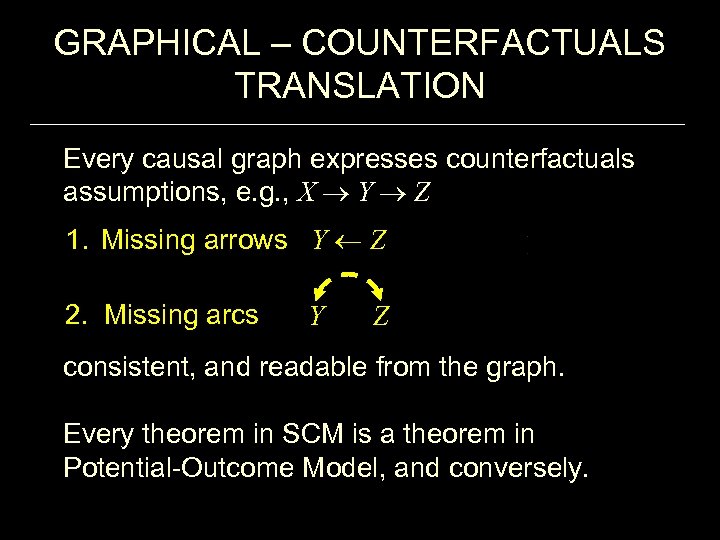 GRAPHICAL – COUNTERFACTUALS TRANSLATION Every causal graph expresses counterfactuals assumptions, e. g. , X Y Z 1. Missing arrows Y Z 2. Missing arcs Y Z consistent, and readable from the graph. Every theorem in SCM is a theorem in Potential-Outcome Model, and conversely.
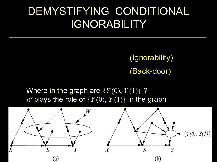 DEMYSTIFYING CONDITIONAL IGNORABILITY (Ignorability) (Back-door) Where in the graph are {Y (0), Y (1)} ? W plays the role of {Y (0), Y (1)} in the graph
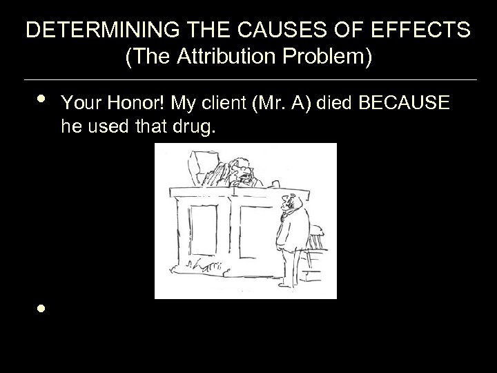 DETERMINING THE CAUSES OF EFFECTS (The Attribution Problem) • Your Honor! My client (Mr. A) died BECAUSE he used that drug. •
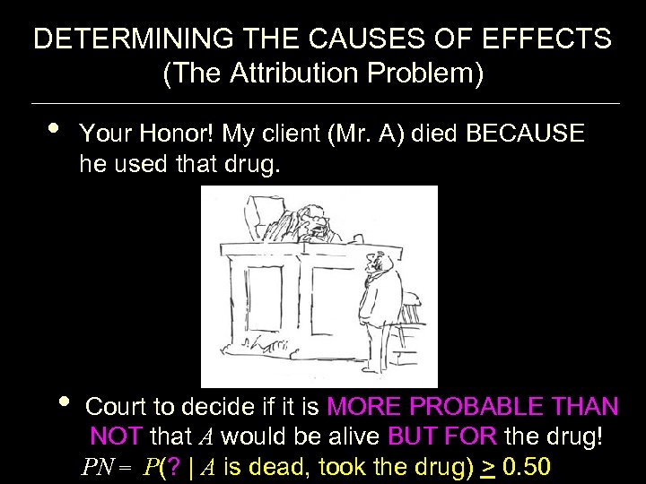 DETERMINING THE CAUSES OF EFFECTS (The Attribution Problem) • Your Honor! My client (Mr. A) died BECAUSE he used that drug. • Court to decide if it is MORE PROBABLE THAN NOT that A would be alive BUT FOR the drug! PN = P(? | A is dead, took the drug) > 0. 50
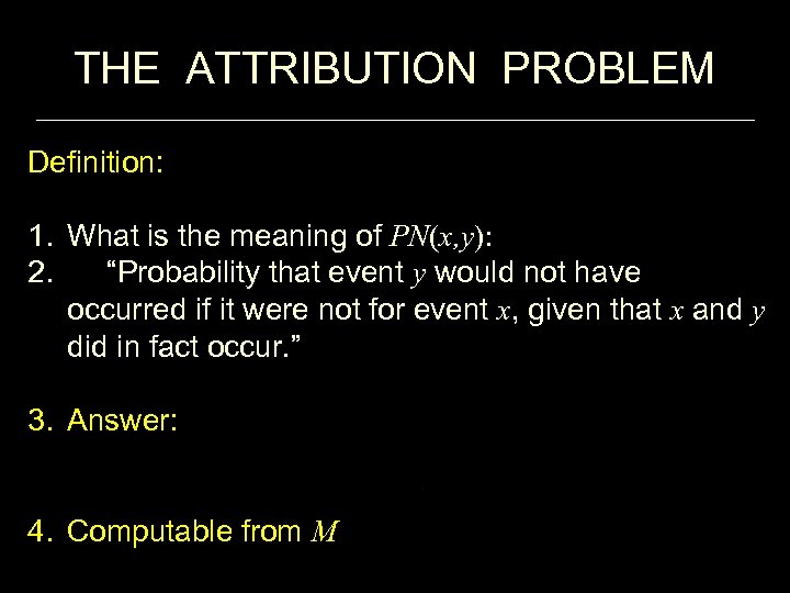 THE ATTRIBUTION PROBLEM Definition: 1. What is the meaning of PN(x, y): 2. “Probability that event y would not have occurred if it were not for event x, given that x and y did in fact occur. ” 3. Answer: 4. Computable from M
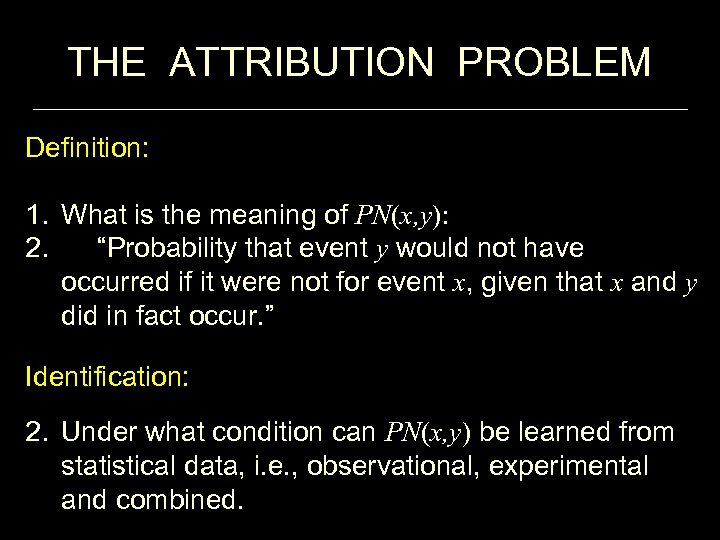 THE ATTRIBUTION PROBLEM Definition: 1. What is the meaning of PN(x, y): 2. “Probability that event y would not have occurred if it were not for event x, given that x and y did in fact occur. ” Identification: 2. Under what condition can PN(x, y) be learned from statistical data, i. e. , observational, experimental and combined.
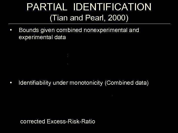 PARTIAL IDENTIFICATION (Tian and Pearl, 2000) • Bounds given combined nonexperimental and experimental data • Identifiability under monotonicity (Combined data) corrected Excess-Risk-Ratio
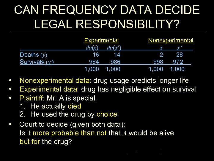 CAN FREQUENCY DATA DECIDE LEGAL RESPONSIBILITY? Deaths (y) Survivals (y ) Experimental do(x) do(x ) 16 14 986 1, 000 Nonexperimental x x 2 28 998 972 1, 000 • Nonexperimental data: drug usage predicts longer life • Experimental data: drug has negligible effect on survival • Plaintiff: Mr. A is special. 1. He actually died 2. He used the drug by choice • Court to decide (given both data): Is it more probable than not that A would be alive but for the drug?
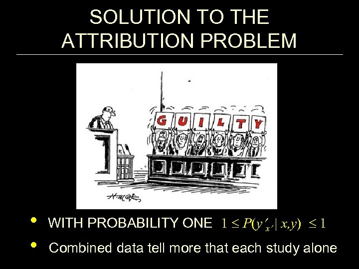 SOLUTION TO THE ATTRIBUTION PROBLEM • WITH PROBABILITY ONE 1 P(y x | x, y) 1 • Combined data tell more that each study alone
 EFFECT DECOMPOSITION (direct vs. indirect effects) 1. Why decompose effects? 2. What is the definition of direct and indirect effects? 3. What are the policy implications of direct and indirect effects? 4. When can direct and indirect effect be estimated consistently from experimental and nonexperimental data?
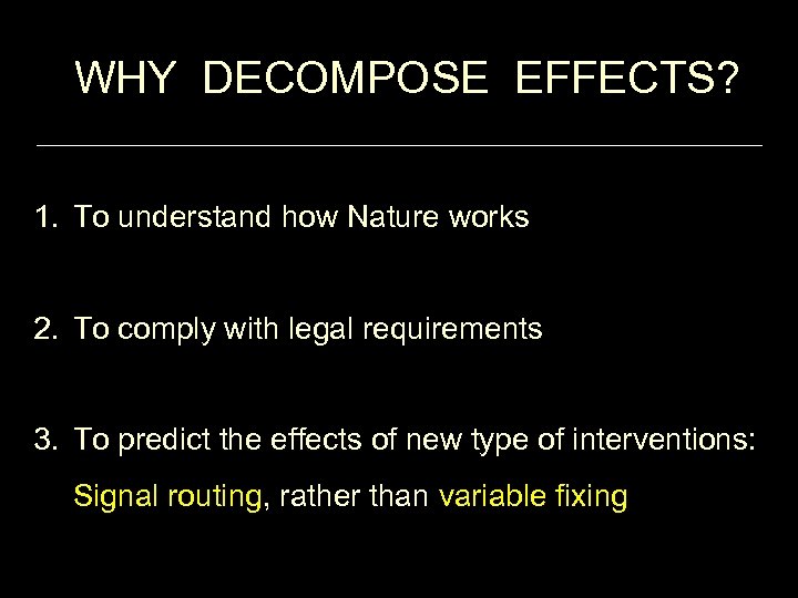 WHY DECOMPOSE EFFECTS? 1. To understand how Nature works 2. To comply with legal requirements 3. To predict the effects of new type of interventions: Signal routing, rather than variable fixing
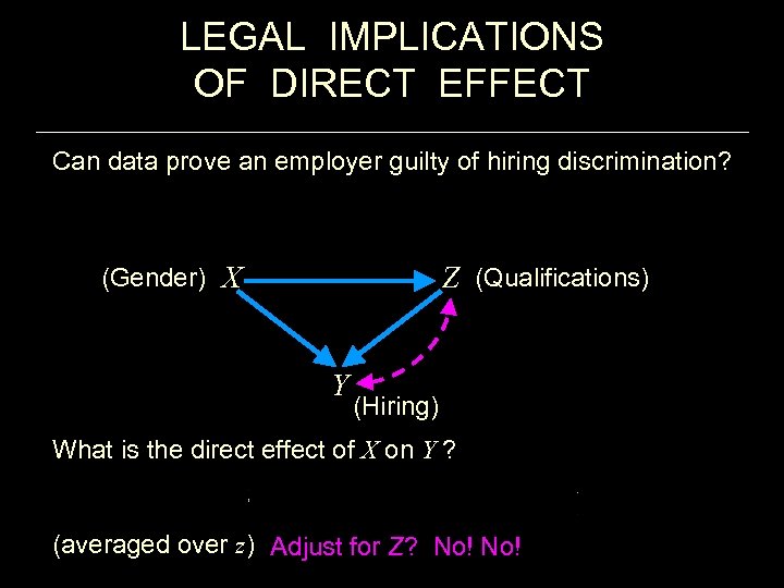 LEGAL IMPLICATIONS OF DIRECT EFFECT Can data prove an employer guilty of hiring discrimination? (Gender) X Z (Qualifications) Y (Hiring) What is the direct effect of X on Y ? (averaged over z) Adjust for Z? No!
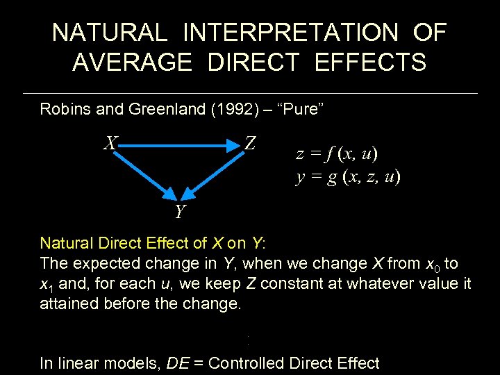 NATURAL INTERPRETATION OF AVERAGE DIRECT EFFECTS Robins and Greenland (1992) – “Pure” X Z z = f (x, u) y = g (x, z, u) Y Natural Direct Effect of X on Y: The expected change in Y, when we change X from x 0 to x 1 and, for each u, we keep Z constant at whatever value it attained before the change. In linear models, DE = Controlled Direct Effect
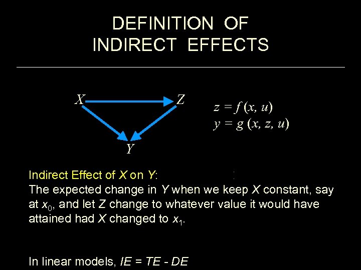 DEFINITION OF INDIRECT EFFECTS X Z z = f (x, u) y = g (x, z, u) Y Indirect Effect of X on Y: The expected change in Y when we keep X constant, say at x 0, and let Z change to whatever value it would have attained had X changed to x 1. In linear models, IE = TE - DE
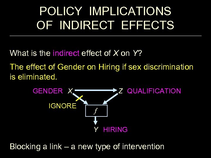 POLICY IMPLICATIONS OF INDIRECT EFFECTS What is the indirect effect of X on Y? The effect of Gender on Hiring if sex discrimination is eliminated. GENDER X IGNORE Z QUALIFICATION f Y HIRING Blocking a link – a new type of intervention
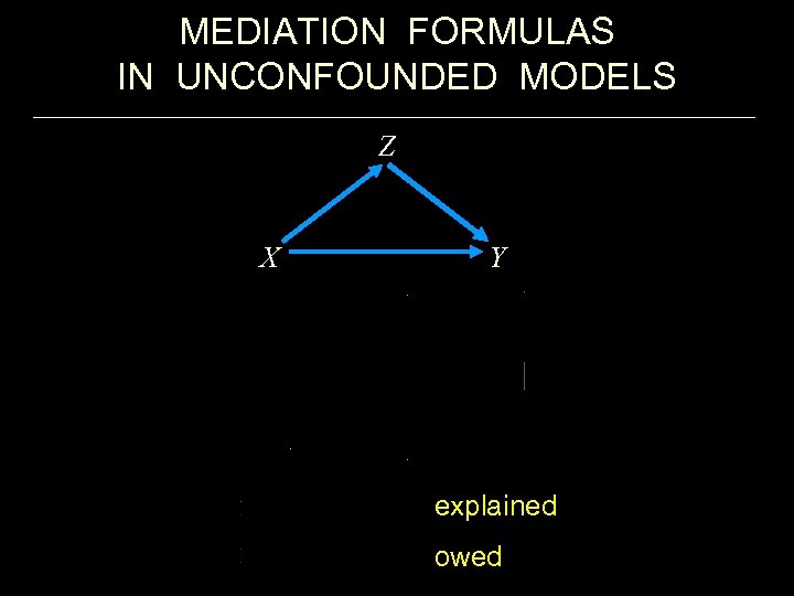 MEDIATION FORMULAS IN UNCONFOUNDED MODELS Z X Y explained owed
 SUMMARY OF MEDIATION RESULTS 1. Formal semantics of path-specific effects, based on disabling mechanisms, instead of value fixing. 2. Path-analytic techniques extended to nonlinear and nonparametric models. 3. Meaningful (graphical) conditions for estimating direct and indirect effects from experimental and nonexperimental data.
 EXTERNAL VALIDITY From Threats to Licenses • • “`External validity’ asks the question of generalizability: To what population, settings, treatment variables, and measurement variables can this effect be generalized? ” (Shadish, Cook and Campbell 2002) “An experiment is said to have `external validity’ if the distribution of outcomes realized by a treatment group is the same as the distribution of outcome that would be realized in an actual program. ” (Manski, 2007) "A threat to external validity is an explanation of how you might be wrong in making a generalization. " (Wikipedia 2011, after Trochin) “A license of validity is a set of theoretical assumptions that neutralizes all conceivable threats. ” (Anon, 2011)
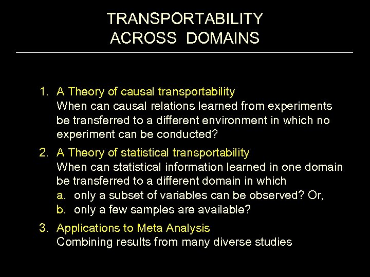 TRANSPORTABILITY ACROSS DOMAINS 1. A Theory of causal transportability When causal relations learned from experiments be transferred to a different environment in which no experiment can be conducted? 2. A Theory of statistical transportability When can statistical information learned in one domain be transferred to a different domain in which a. only a subset of variables can be observed? Or, b. only a few samples are available? 3. Applications to Meta Analysis Combining results from many diverse studies
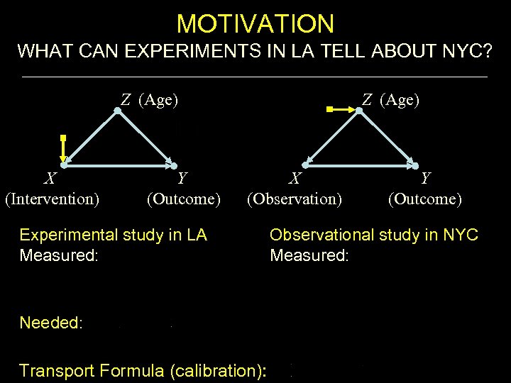 MOTIVATION WHAT CAN EXPERIMENTS IN LA TELL ABOUT NYC? Z (Age) X (Intervention) Y (Outcome) Z (Age) X (Observation) Experimental study in LA Measured: Needed: Transport Formula (calibration): Y (Outcome) Observational study in NYC Measured:
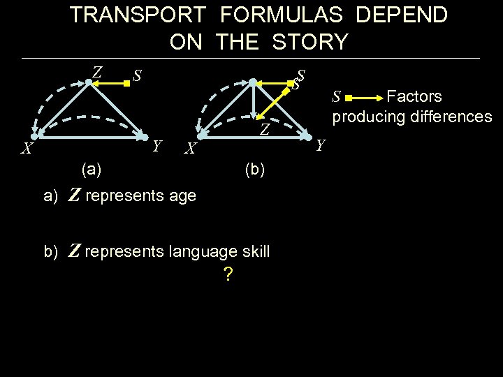 TRANSPORT FORMULAS DEPEND ON THE STORY Z S S S Y X Z X (a) (b) a) Z represents age b) Z represents language skill ? S Factors producing differences Y
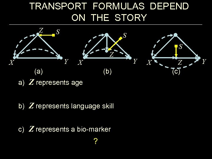 TRANSPORT FORMULAS DEPEND ON THE STORY Z S S S Y X Z X (a) (b) a) Z represents age b) Z represents language skill c) Z represents a bio-marker ? Y X Z (c) Y
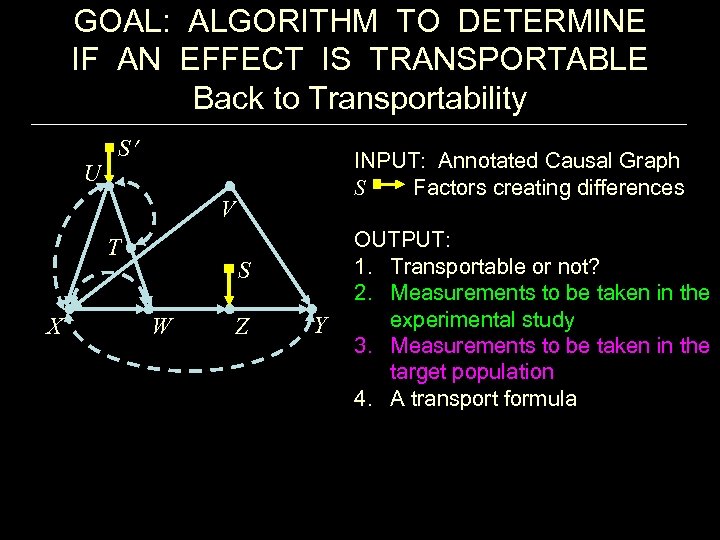 GOAL: ALGORITHM TO DETERMINE IF AN EFFECT IS TRANSPORTABLE Back to Transportability U S V T X S W Z Y INPUT: Annotated Causal Graph S Factors creating differences OUTPUT: 1. Transportable or not? 2. Measurements to be taken in the experimental study 3. Measurements to be taken in the target population 4. A transport formula
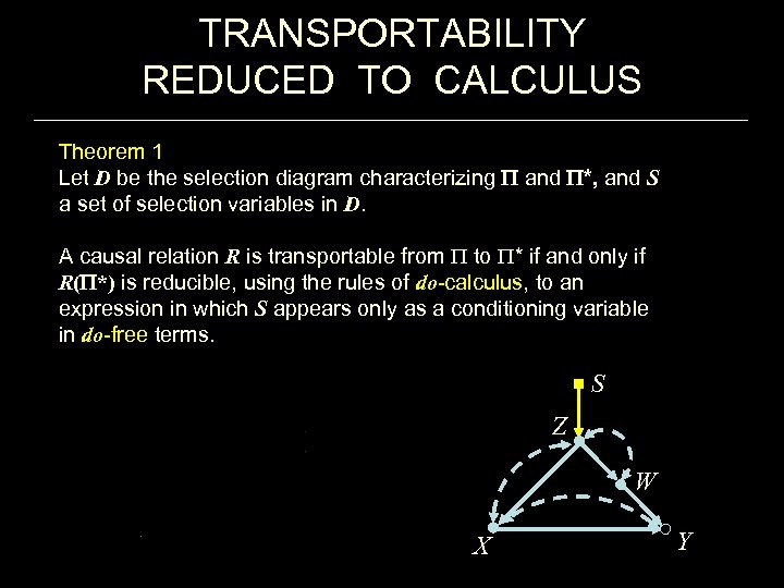 TRANSPORTABILITY REDUCED TO CALCULUS Theorem 1 Let D be the selection diagram characterizing and *, and S a set of selection variables in D. A causal relation R is transportable from to * if and only if R( *) is reducible, using the rules of do-calculus, to an expression in which S appears only as a conditioning variable in do-free terms. S Z W X Y
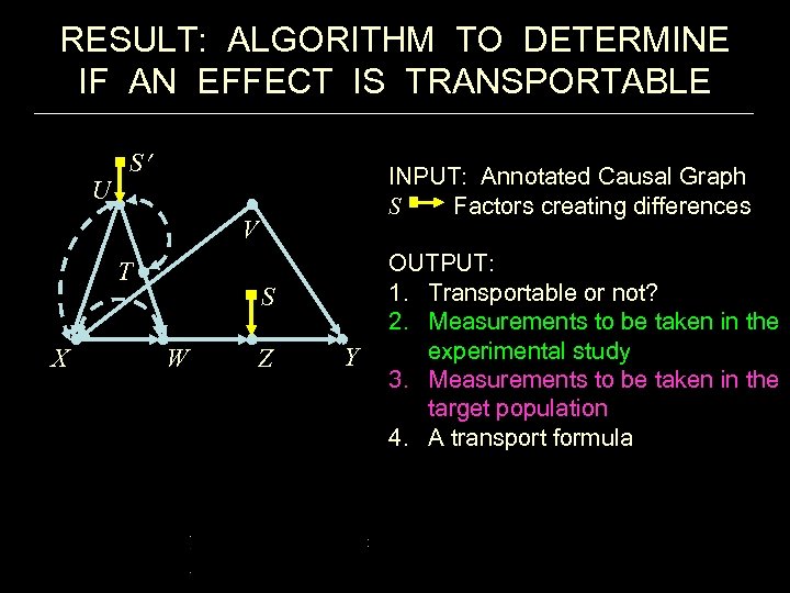 RESULT: ALGORITHM TO DETERMINE IF AN EFFECT IS TRANSPORTABLE U S V T X S W Z Y INPUT: Annotated Causal Graph S Factors creating differences OUTPUT: 1. Transportable or not? 2. Measurements to be taken in the experimental study 3. Measurements to be taken in the target population 4. A transport formula
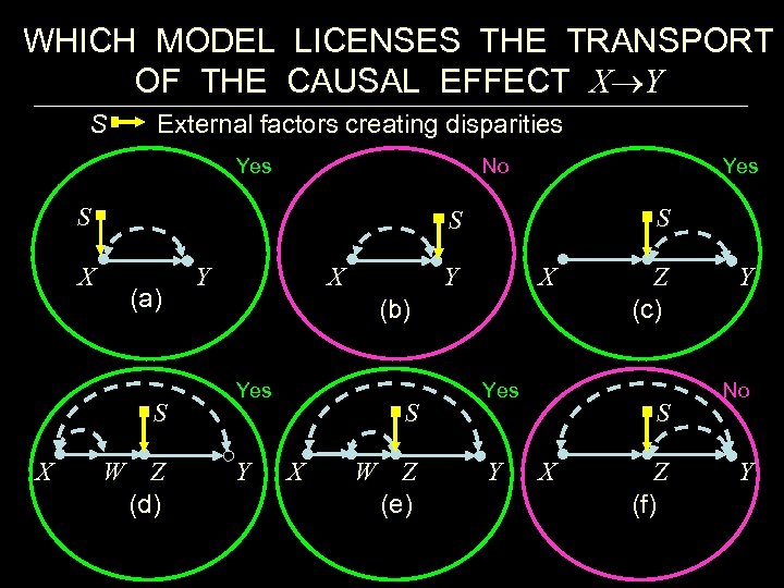 WHICH MODEL LICENSES THE TRANSPORT OF THE CAUSAL EFFECT X Y S External factors creating disparities Yes No S X S S (a) S X Yes W Z (d) X Y Y X (b) Yes Y S X W Z (e) Yes Y Z (c) S X Z (f) Y No Y
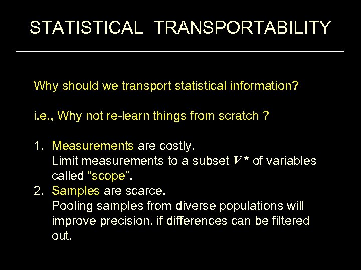 STATISTICAL TRANSPORTABILITY Why should we transport statistical information? i. e. , Why not re-learn things from scratch ? 1. Measurements are costly. Limit measurements to a subset V * of variables called “scope”. 2. Samples are scarce. Pooling samples from diverse populations will improve precision, if differences can be filtered out.
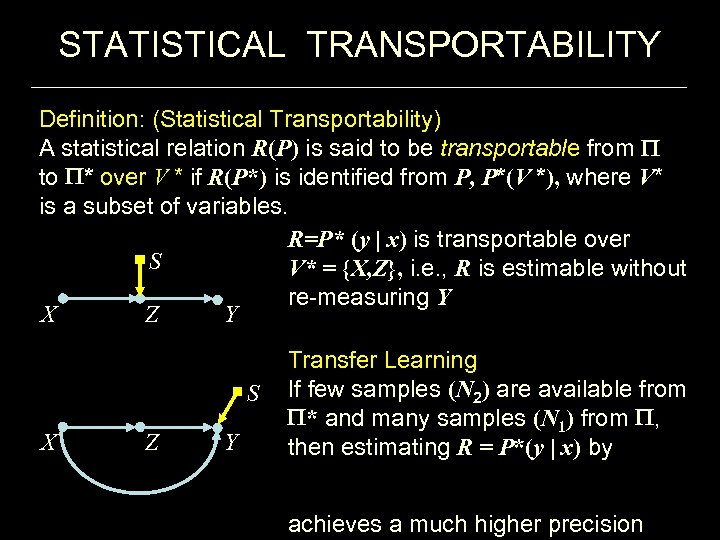 STATISTICAL TRANSPORTABILITY Definition: (Statistical Transportability) A statistical relation R(P) is said to be transportable from to * over V * if R(P*) is identified from P, P*(V *), where V* is a subset of variables. R=P* (y | x) is transportable over S V* = {X, Z}, i. e. , R is estimable without re-measuring Y X Z Y S X Z Y Transfer Learning If few samples (N 2) are available from * and many samples (N 1) from , then estimating R = P*(y | x) by achieves a much higher precision
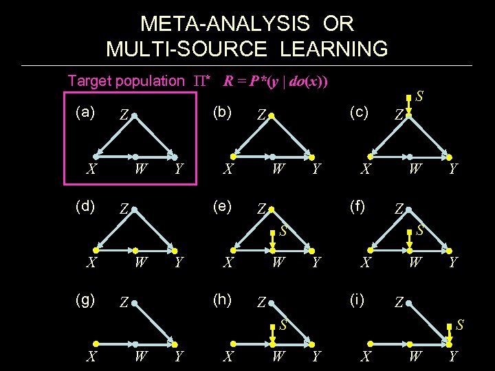 META-ANALYSIS OR MULTI-SOURCE LEARNING Target population * R = P*(y | do(x)) (a) X (d) (b) Z W Y X (e) Z (c) Z W Y Z X (f) Z S W Z S S X (g) W Y X (h) Z W Y X (i) Z W W Y X W Y Z S S X Y Y X W Y
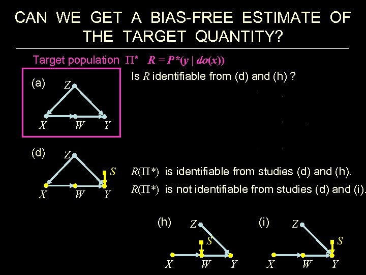 CAN WE GET A BIAS-FREE ESTIMATE OF THE TARGET QUANTITY? Target population * R = P*(y | do(x)) Is R identifiable from (d) and (h) ? (a) Z X (d) W Y Z S R( *) is identifiable from studies (d) and (h). X W Y R( *) is not identifiable from studies (d) and (i). (h) (i) Z Z S S X W Y
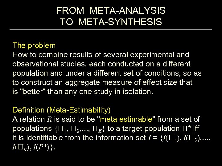 FROM META-ANALYSIS TO META-SYNTHESIS The problem How to combine results of several experimental and observational studies, each conducted on a different population and under a different set of conditions, so as to construct an aggregate measure of effect size that is "better" than any one study in isolation. Definition (Meta-Estimability) A relation R is said to be "meta estimable" from a set of populations { 1, 2, . . . , K} to a target population * iff it is identifiable from the information set I = {I( 1), I( 2), . . . , I( K), I(P*)}.
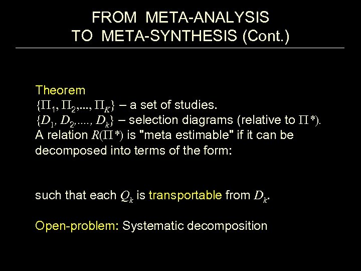 FROM META-ANALYSIS TO META-SYNTHESIS (Cont. ) Theorem { 1, 2, . . . , K} – a set of studies. {D 1, D 2, . . , Dk} – selection diagrams (relative to *). A relation R( *) is "meta estimable" if it can be decomposed into terms of the form: such that each Qk is transportable from Dk. Open-problem: Systematic decomposition
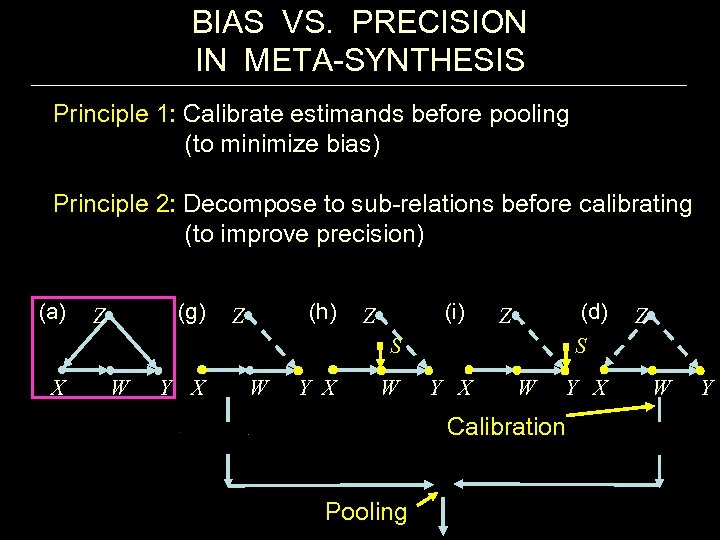 BIAS VS. PRECISION IN META-SYNTHESIS Principle 1: Calibrate estimands before pooling (to minimize bias) Principle 2: Decompose to sub-relations before calibrating (to improve precision) (a) (g) Z (h) Z (i) Z (d) Z S X W Y X W S Y X W Y X Calibration Pooling Z W Y
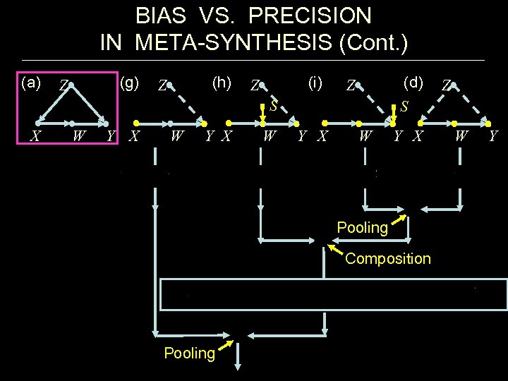 BIAS VS. PRECISION IN META-SYNTHESIS (Cont. ) (a) (g) Z (h) Z (i) Z (d) Z S X W Y X W S Y X W Y X Pooling Composition Pooling Z W Y
 CONCLUSIONS I TOLD YOU CAUSALITY IS SIMPLE • Principled methodology for causal and counterfactual inference (complete) • Unification of the graphical, potential-outcome and structural equation approaches • Friendly and formal solutions to century-old problems and confusions.
 CONCLUSIONS He is wise who bases causal inference on an explicit causal structure that is defensible on scientific grounds. (Aristotle 384 -322 B. C. ) From Charlie Poole
 QUESTIONS? ? ? Now is the time!


