9d5e429c1b8a78bb4da7313d2902f474.ppt
- Количество слайдов: 123
Carnegie Mellon Bio. War Center for Computational Analysis of Social and Organizational Systems Institute for Software Research International Kathleen M. Carley Project Director Carnegie Mellon University Wean 1323 Pittsburgh, PA 15213 Tel: 1 -412 -268 -6016 Fax: 1412 -268 -1744 Email: kathleen. carley@cmu. edu 2003 1
POC Bio. War – Project Director and PI Kathleen M. Carley Wean 1323 Institute for Software Research International, SCS Carnegie Mellon University Pittsburgh, PA 15213 Tel: 412 -268 -6016 Fax: 412 -268 -2338 Email: kathleen. carley@cmu. edu Web: http: //www. casos. ece. cmu. edu/bios/carley/bio_carley. html May 2003 © Kathleen M. Carley – Carnegie Mellon – ISRI, CASOS 2
Bio. War Project Team – March 2003 ¯ ¯ ¯ Bio. War – Project Director and PI Kathleen M. Carley, ISRI, Ph. D. Doug Fridsma – University of Pittsburgh, BMSI, Ph. D. M. D. David Deerfield – PSC, Director of Biomedical Initiative, Ph. D. Liz Casman – CMU, EPP, research scientist Graduate Students ¯ Alex Yaja, ISRI ¯ Programming Staff ¯ Boris Kaminsky, ISRI, Ph. D. ¯ Démian Nave, PSC, MSCS. ¯ Neal Altman, ISRI, MSCS. ¯ Previous Support ¯ Natasha Kamneva, ISRI, ¯ Jack Chang, PSC, Ph. D. ¯ Summer Support for Validation and Collection of Disease Data ¯ Tiffany Tummino, grad student ¯ Li-Chiou Chen, grad student May 2003 © Kathleen M. Carley – Carnegie Mellon – ISRI, CASOS 3
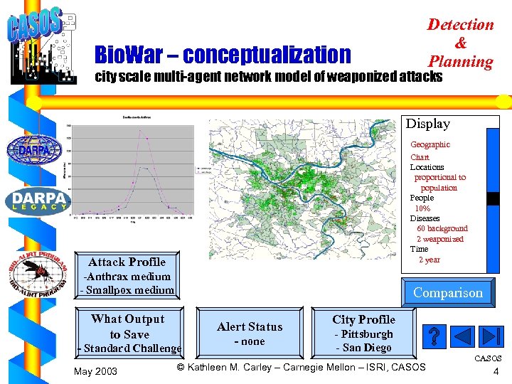
Detection & Planning Bio. War – conceptualization city scale multi-agent network model of weaponized attacks Display Geographic Chart Locations proportional to population People 10% Diseases 60 background 2 weaponized Time 2 year Attack Profile -Anthrax medium - Smallpox medium Comparison What Output to Save Alert Status - Standard Challenge May 2003 - none City Profile - Pittsburgh - San Diego © Kathleen M. Carley – Carnegie Mellon – ISRI, CASOS 4
Bio. War Objective ¯ Automated tool ¯ for evaluation of response policies, data efficacy, attack severity, and detection tools relating to weaponized biological attacks ¯ for estimating spread of disease due to infection or aerosolized release ¯ Enables user to systematically and automatically reason about: ¯ ¯ The rate and spread of disease with high degree of realism Early presentation of diseases Potential media and inoculation campaigns (cost, benefit, effectiveness) Other “what-if” occurrence, early detection, and response scenarios ¯ Enables the design of policies for bio-response ¯ ¯ ¯ For weaponized and non-weaponized outbreaks Timing and efficacy of alerts Effectiveness of inoculation strategies Cost-effectiveness of a policy Automated evaluation of response policy and prediction of its outcomes May 2003 © Kathleen M. Carley – Carnegie Mellon – ISRI, CASOS 5
Potential Usage ¯ Generate possible attacks – ¯ As a data layer added to existing data ¯ As a data layer for some outputs (such as ER) and full data for other variables (such as OTC purchases) ¯ As a complete city simulation (all data not just attack) ¯ ¯ ¯ Examine effectiveness/costliness of response policies Examine effectiveness of containment policies Creation of dynamic gaming environment Pre-evaluate possible types of data sets for detection Pre-evaluate using empirically validated simulated data whether more detailed data collection might be useful ¯ Training for intel officers and health workers about what an attack might look like May 2003 © Kathleen M. Carley – Carnegie Mellon – ISRI, CASOS 6
Approach ¯ Multi-Agent Network Model ¯ ¯ ¯ Cognitively realistic Socially realistic – embedded in social, knowledge, and task networks Spatio-temporally realistic Organizational network Communication technologies ¯ Hybrid of many models – Modular design ¯ Agent – Social network – Behavioral response ¯ Disease ¯ City – Population – Site locations ¯ Cost ¯ Media ¯ Weather ¯ … May 2003 © Kathleen M. Carley – Carnegie Mellon – ISRI, CASOS 7
Why Agent-based simulation of disease? ¯ General-purpose approach to eliminating “homogeneous mixing” assumption ¯ Social networks provide mechanism for population mixing on arbitrary number of parameters ¯ Stochastic nature of the model can generate “unpredictable outcomes” with interaction effects ¯ Allows modeling at multiple levels (dispersion, response, disease, diagnosis, etc) since agent is common across all of these models ¯ Particularly useful for contagious diseases (SARS, smallpox) ¯ Particularly useful for examining detection potential of DNA hybridization techniques May 2003 © Kathleen M. Carley – Carnegie Mellon – ISRI, CASOS 8
Implementation ¯ ¯ Social network multi-agent system Data for three metro-areas (census (business and population), weather) V 1 26, 000 agents, 10 diseases, 2 years, 100’s locations in 5 hours V 2 (used for C 2) 260, 000 agents, 60 diseases, 5 years, 1000 s locations in 1 hour (PC & Unix version) ¯ V 2. 1 (used for C 3) 562, 000 agents, 60 diseases, 2 years, 10, 000 s locations, 6. 5 hours, 4 processors (Unix& PC is forthcoming) ¯ Length of run impacted by: ¯ C 1 by number of agents, locations, diseases ¯ C 2/3 only significantly by number of agents ¯ Geometry grid – latitude/longitude (perlscript to convert to UTM) ¯ Data reporting lags (based on real data) ¯ Existing output streams (CSV format) ¯ ¯ ¯ Over the counter purchases (5 categories) School/work capacity & attendance (absenteeism matches real) Web lookups and phone calls (too low) Doctor, ER (matches real for flu) EPIs per disease ¯ Validation at mean level for each output behavior ¯ Batch operation May 2003 © Kathleen M. Carley – Carnegie Mellon – ISRI, CASOS 9
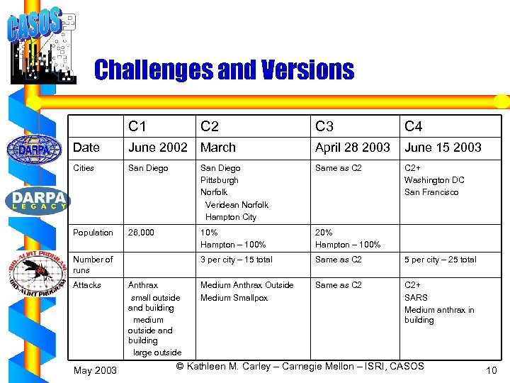
Challenges and Versions C 1 C 2 C 3 C 4 Date June 2002 March April 28 2003 June 15 2003 Cities San Diego Pittsburgh Norfolk Veridean Norfolk Hampton City Same as C 2+ Washington DC San Francisco Population 26, 000 10% Hampton – 100% 20% Hampton – 100% 3 per city – 15 total Same as C 2 5 per city – 25 total Medium Anthrax Outside Medium Smallpox Same as C 2+ SARS Medium anthrax in building Number of runs Attacks May 2003 Anthrax small outside and building medium outside and building large outside © Kathleen M. Carley – Carnegie Mellon – ISRI, CASOS 10
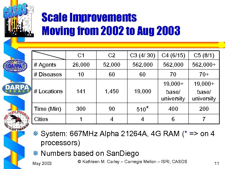
Scale Improvements Moving from 2002 to Aug 2003 C 1 # Agents # Diseases C 2 C 3 (4/ 30) C 4 (6/15) C 5 (8/1) 26, 000 52, 000 562, 000+ 10 60 60 70 70+ 19, 000+ base/ university # Locations 141 1, 450 19, 000+ base/ university Time (Min) 300 90 510* 400 200 1 4 4 6 7 Cities ¯ System: 667 MHz Alpha 21264 A, 4 G RAM (* => on 4 processors) ¯ Numbers based on San. Diego May 2003 © Kathleen M. Carley – Carnegie Mellon – ISRI, CASOS 11
Near Term Development Plans ¯ June 15 ¯ ¯ ¯ ¯ Add two more cities – San Francisco and DC Add universities In building attacks Increased activities/ticks Impact of inoculation, random, inoculation of med personnel Symptom based treatment Improve robustness of disease model Improve baseline disease fidelity and distractors – E. g. , by adding accidents and heart attacks ¯ Aug 1 ¯ Examination of what % of city needs to be modeled as agents to get overall impact and correct cross-correlations for behavior ¯ Webhits and phone calls from home and work ¯ All 7 weaponized disease, SARS ¯ Complete Base Model for Norfolk ¯ Ability to layer data on Pavlin Mil. data and/or create complimentary files for other data streams (need data this month to meet this goal) ¯ Layering for Pavlin Mil. Base data May 2003 © Kathleen M. Carley – Carnegie Mellon – ISRI, CASOS 12
Longer Term Development Plans & Desired Features ¯ Post Aug 1 ¯ Change behavior of agents based on diagnosis of weaponized disease ¯ Possible panic model – by lowering evoking strength ¯ Additional data streams – e. g. , 911, temperature, water usage ¯ Possible new studies ¯ Contrast syndromic surveillance with DNA hybridization technique – Help evaluate value of symptom based data streams versus pathogen data streams ¯ Non-Linear scaling procedures – How to scale x% of the agents, locations, acreage to look like the entire city ¯ Desired Features ¯ ¯ For $50, 000 we could raise this to 600 diseases For $25, 000 we could test attachment to HPAC on new city For $70, 000 we could link to Arcview for improved spatial modeling Integrate with “heavy duty” database – oracle. May 2003 © Kathleen M. Carley – Carnegie Mellon – ISRI, CASOS 13
Linkage to Bio-Alirt Efforts ¯ Generating data samples for Veridian ¯ Building new modules as requested by groups ¯ Survey, web hits, extended OTC, ¯ Built/building metro areas as requested by various groups ¯ ¯ ¯ Pittsburgh San Diego Norfolk Pavlin’s Mil. Base in Norfolk San Francisco Washington D. C. ¯ Providing information & references for inject group ¯ Providing lessons learned on how to inject data ¯ Augmenting Bio. War to generate inject data for Pavlin Mil. Base data ¯ Possible development of a simulated “virtual-ville” for examination of privacy issues May 2003 © Kathleen M. Carley – Carnegie Mellon – ISRI, CASOS 14
Usage of Bio. War Beyond This Program ¯ Usage by Army and contractors for providing data for testing their detection routines ¯ Current discussions with AFRL ¯ Possible test for NYC – if can link to HPAC ¯ Possible partnership with Toronto health group for estimating impact of SARS ¯ Utilization of Bio. War to examine spread of sexually transmitted diseases ¯ DSTO in Australia is potentially interested in using Bio. War ¯ Limitations on use: ¯ ¯ Apx. 1 -3 months to set up new US city Data output should be to database such as oracle Multi-processor system speeds execution May require substantial changes to parameters for non US May 2003 © Kathleen M. Carley – Carnegie Mellon – ISRI, CASOS 15
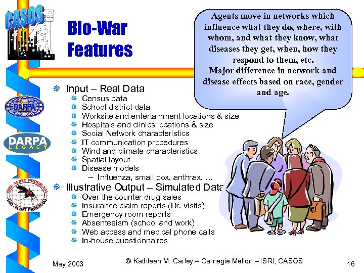
Bio-War Features ¯ Input – Real Data ¯ ¯ ¯ ¯ ¯ Agents move in networks which influence what they do, where, with whom, and what they know, what diseases they get, when, how they respond to them, etc. Major difference in network and disease effects based on race, gender and age. Census data School district data Worksite and entertainment locations & size Hospitals and clinics locations & size Social Network characteristics IT communication procedures Wind and climate characteristics Spatial layout Disease models – Influenza, small pox, anthrax, … ¯ Illustrative Output – Simulated Data ¯ ¯ ¯ Over the counter drug sales Insurance claim reports (Dr. visits) Emergency room reports Absenteeism (school and work) Web access and medical phone calls In-house questionnaires May 2003 © Kathleen M. Carley – Carnegie Mellon – ISRI, CASOS 16
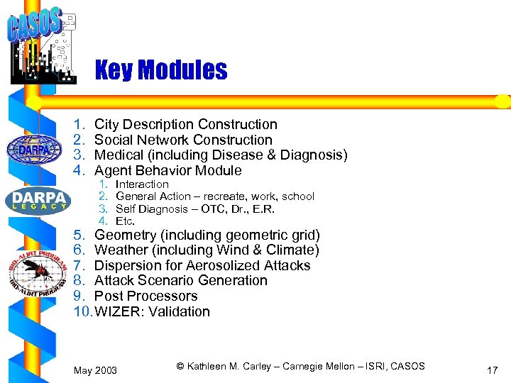
Key Modules 1. 2. 3. 4. City Description Construction Social Network Construction Medical (including Disease & Diagnosis) Agent Behavior Module 1. 2. 3. 4. Interaction General Action – recreate, work, school Self Diagnosis – OTC, Dr. , E. R. Etc. 5. Geometry (including geometric grid) 6. Weather (including Wind & Climate) 7. Dispersion for Aerosolized Attacks 8. Attack Scenario Generation 9. Post Processors 10. WIZER: Validation May 2003 © Kathleen M. Carley – Carnegie Mellon – ISRI, CASOS 17
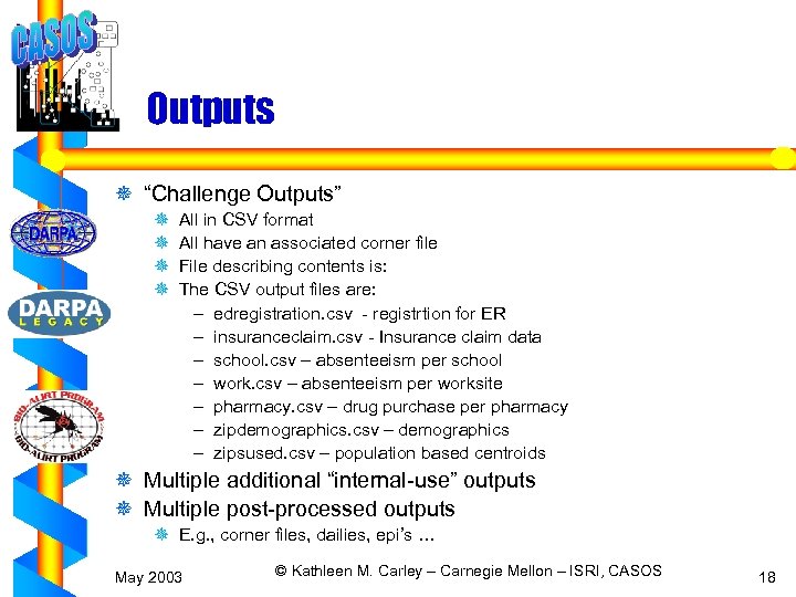
Outputs ¯ “Challenge Outputs” ¯ ¯ All in CSV format All have an associated corner file File describing contents is: The CSV output files are: – edregistration. csv - registrtion for ER – insuranceclaim. csv - Insurance claim data – school. csv – absenteeism per school – work. csv – absenteeism per worksite – pharmacy. csv – drug purchase per pharmacy – zipdemographics. csv – demographics – zipsused. csv – population based centroids ¯ Multiple additional “internal-use” outputs ¯ Multiple post-processed outputs ¯ E. g. , corner files, dailies, epi’s … May 2003 © Kathleen M. Carley – Carnegie Mellon – ISRI, CASOS 18
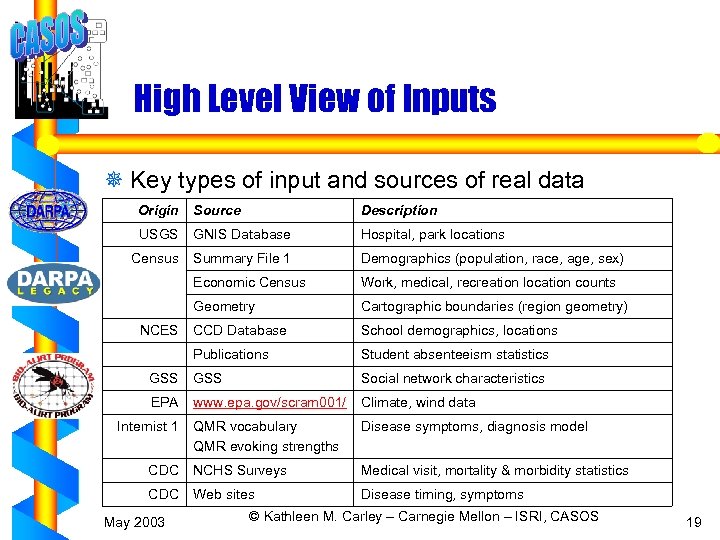
High Level View of Inputs ¯ Key types of input and sources of real data Origin Source Description USGS GNIS Database Hospital, park locations Census Summary File 1 Demographics (population, race, age, sex) Economic Census Work, medical, recreation location counts Geometry Cartographic boundaries (region geometry) CCD Database School demographics, locations Publications Student absenteeism statistics GSS Social network characteristics EPA www. epa. gov/scram 001/ Climate, wind data QMR vocabulary QMR evoking strengths Disease symptoms, diagnosis model CDC NCHS Surveys Medical visit, mortality & morbidity statistics CDC Web sites Disease timing, symptoms NCES Internist 1 May 2003 © Kathleen M. Carley – Carnegie Mellon – ISRI, CASOS 19
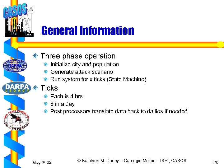
General Information ¯ Three phase operation ¯ Initialize city and population ¯ Generate attack scenario ¯ Run system for x ticks (State Machine) ¯ Ticks ¯ Each is 4 hrs ¯ 6 in a day ¯ Post processors translate data back to dailies if needed May 2003 © Kathleen M. Carley – Carnegie Mellon – ISRI, CASOS 20
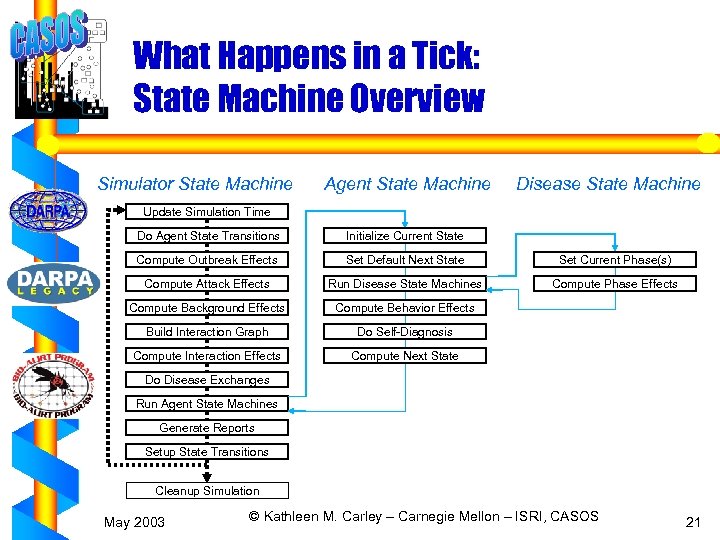
What Happens in a Tick: State Machine Overview Simulator State Machine Agent State Machine Disease State Machine Update Simulation Time Do Agent State Transitions Initialize Current State Compute Outbreak Effects Set Default Next State Set Current Phase(s) Compute Attack Effects Run Disease State Machines Compute Phase Effects Compute Background Effects Compute Behavior Effects Build Interaction Graph Do Self-Diagnosis Compute Interaction Effects Compute Next State Do Disease Exchanges Run Agent State Machines Generate Reports Setup State Transitions Cleanup Simulation May 2003 © Kathleen M. Carley – Carnegie Mellon – ISRI, CASOS 21
Module 1: City Description Construction ¯ City construction initializes geometry, demographics, agent definitions, and other inputs for one or more simulation runs ¯ Process overview (“gensim” that utilizes real data): ¯ Load configuration file (sets city scale, calendar range, etc. ) ¯ Load global data (disease data, generic statistics, etc. ) ¯ Load city data (geometry, population & school demographics, location positions and sizes, weather system, attack and outbreak specs, etc. ) ¯ Generate city (random population, agent social network, locations, jobs & schools, outbreak and attack calendar, weather calendar, etc. ) ¯ Inputs generated for simulator (“Bio. War”’s Simulated City) ¯ Population and infrastructure (properly-distributed agents, jobs, schools, entertainment locations) ¯ Simulator data (social network, weather calendar, attack & outbreak instance characteristics) ¯ Note: generated cities are saved enabling multiple runs on same city May 2003 © Kathleen M. Carley – Carnegie Mellon – ISRI, CASOS 22
Module 1: City Construction (Cont’d)— Random Population ¯ Per-census tract demographics for simulation region are extracted from locally installed Census database ¯ Simulated Agents are assigned to tracts by throwing a random die R in [0, 1] against a cumulative probability distribution over tract population ¯ Simulated Agent profiles are similarly generated using cumulative distributions over the per-tract demographic profiles May 2003 © Kathleen M. Carley – Carnegie Mellon – ISRI, CASOS 23
Module 1: City Construction (Cont’d)—Ego Net and Home Generation ¯ Actual census tract assignments are then used to guide the generation of ego networks for simulated families ¯ Simulated family ego nets are used to determine “cohabitating agents” ¯ Simulated cohabitating agents are then assigned to the same home location (affects job and school assignment) May 2003 © Kathleen M. Carley – Carnegie Mellon – ISRI, CASOS 24
Module 1: City Construction (Cont’d)— School Generation and Assignment ¯ Actual per-school demographics are extracted from a locally-installed NCES CCD dataset (public schools only) ¯ Simulated schools are mapped to the districts that contain them (schools are guaranteed to have a district) ¯ Simulated agents with homes in each school district are then assigned randomly by age to a simulated school in that district May 2003 © Kathleen M. Carley – Carnegie Mellon – ISRI, CASOS 25
Module 1: City Construction (Cont’d)— City Infrastructure Generation ¯ City infrastructure currently consists of locations only (some random, some specified by a GNIS database) ¯ Positions of jobs, doctors, pharmacies, restaurants, stores, & theaters generated randomly, with capacities from a NAICS database ¯ Positions of simulated hospitals and parks are based on the actual using GNIS, capacities from NAICS ¯ Randomly generated positions of simulated locations, such as restaurants, are distributed uniformly over the simulated city based upon actual census tract population and geometry ¯ Simulated agents are currently randomly assigned to jobs May 2003 © Kathleen M. Carley – Carnegie Mellon – ISRI, CASOS 26
Module 1: City Construction (Cont’d)—Other Generated Inputs ¯ Simulated weather calendar (described later) includes wind (for attack resolution) and climate (temperature, pressure, precipitation) ¯ Schedule for simulated outbreaks and attacks based upon user-specified parameters (also described later) May 2003 © Kathleen M. Carley – Carnegie Mellon – ISRI, CASOS 27
Module 1: Data Sources for City Construction ¯ Urban Area Definitions ¯ US Census Bureau - Metropolitan Statistical Areas: 1999 ¯ ZIP Codes – Zip. Express™ – Lookup Zip Codes by County – Capitolimpact. com – Capitolimpact Gateway ¯ US Census Bureau Cartographic Boundary Files ¯ MSA boundaries – Census Tracts: 2000 – 3 -Digit ZIP Code Tabulation Areas (ZCTAs): 2000 – 5 -Digit ZIP Code Tabulation Areas (ZCTAs): 2000 ¯ Schools – School Districts - Elementary: 2000 – School Districts - Secondary: 2000 – School Districts - Unified: 2000 ¯ Location Names, Counts and Geographic Coordinates ¯ US Census Bureau - 2000 Economic Census ¯ NAICS – count of entertainment/recreation, work, doctor, pharmacy locations ¯ GSS – ego net input (indirectly affects number of homes) ¯ USGS – GNIS (Geographic Names Information System) – positions of hospitals, parks & stadiums ¯ NCES – CCD Public School District Data ¯ NCES – CCD Public School Data May 2003 © Kathleen M. Carley – Carnegie Mellon – ISRI, CASOS 28
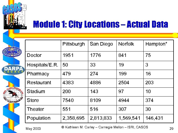
Module 1: City Locations – Actual Data Pittsburgh San Diego Norfolk Hampton* 1951 1776 841 75 Hospitals/E. R. 50 33 19 3 Pharmacy 479 274 199 16 Restaurant 4383 4886 2504 203 Stadium 200 143 97 10 Store 7540 8109 4944 374 Theater 551 516 307 30 Population 2, 358, 695 2, 813, 833 1, 569, 541 146, 431 Doctor May 2003 © Kathleen M. Carley – Carnegie Mellon – ISRI, CASOS 29
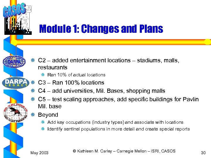
Module 1: Changes and Plans ¯ C 2 – added entertainment locations – stadiums, malls, restaurants ¯ Ran 10% of actual locations ¯ C 3 – Ran 100% locations ¯ C 4 – add universities, Mil. Bases, shopping malls ¯ C 5 – test scaling approaches, add specific buildings for Pavlin Mil. base ¯ Beyond ¯ Add key occupations (industry types) and associate with locations ¯ Identify sentinel populations in more detail and create special reports May 2003 © Kathleen M. Carley – Carnegie Mellon – ISRI, CASOS 30
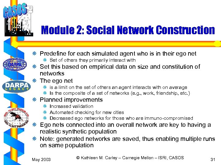
Module 2: Social Network Construction ¯ Predefine for each simulated agent who is in their ego net ¯ Set of others they primarily interact with ¯ Set this based on empirical data on size and constitution of networks ¯ The ego net ¯ is a limit on the set of others an agent interacts with on average ¯ Is the composite of a set of networks (e. g. , work, friendship, etc. ) ¯ Planned improvements ¯ Increased validation ¯ Automated checking for new cities ¯ Decreased ego networks for those who are immuno-compromised ¯ Ego nets connected into an overall network are key to having a realistic synthetic population ¯ Note: generated networks are saved, thus enabling multiple runs on same population May 2003 © Kathleen M. Carley – Carnegie Mellon – ISRI, CASOS 31
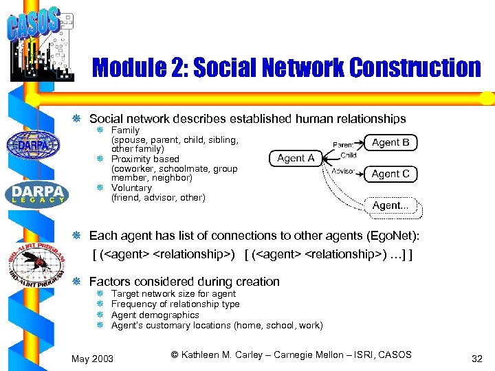
Module 2: Social Network Construction ¯ Social network describes established human relationships ¯ Family (spouse, parent, child, sibling, other family) ¯ Proximity based (coworker, schoolmate, group member, neighbor) ¯ Voluntary (friend, advisor, other) ¯ Each agent has list of connections to other agents (Ego. Net): [ (<agent> <relationship>) …] ] ¯ Factors considered during creation ¯ ¯ Target network size for agent Frequency of relationship type Agent demographics Agent’s customary locations (home, school, work) May 2003 © Kathleen M. Carley – Carnegie Mellon – ISRI, CASOS 32
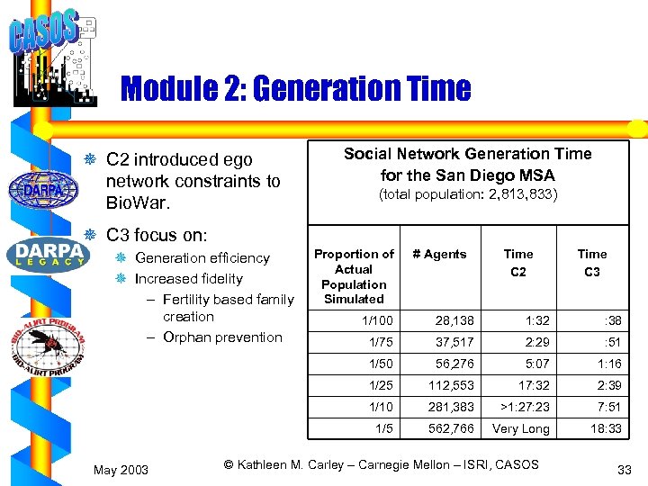
Module 2: Generation Time ¯ C 2 introduced ego network constraints to Bio. War. Social Network Generation Time for the San Diego MSA (total population: 2, 813, 833) ¯ C 3 focus on: ¯ Generation efficiency ¯ Increased fidelity – Fertility based family creation – Orphan prevention Proportion of Actual Population Simulated # Agents Time C 2 Time C 3 28, 138 1: 32 : 38 1/75 37, 517 2: 29 : 51 1/50 56, 276 5: 07 1: 16 1/25 112, 553 17: 32 2: 39 1/10 281, 383 >1: 27: 23 7: 51 1/5 May 2003 1/100 562, 766 Very Long 18: 33 © Kathleen M. Carley – Carnegie Mellon – ISRI, CASOS 33
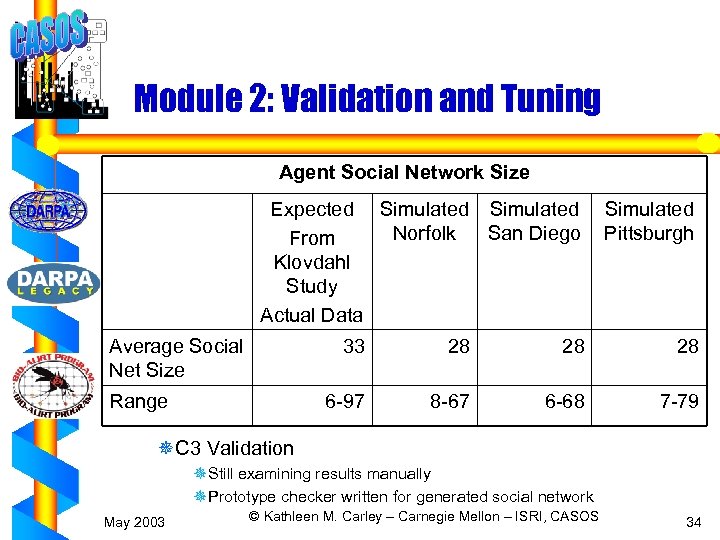
Module 2: Validation and Tuning Agent Social Network Size Expected Simulated Norfolk San Diego From Klovdahl Study Actual Data Average Social Net Size Simulated Pittsburgh 33 28 28 6 -97 Range 28 8 -67 6 -68 7 -79 ¯C 3 Validation ¯Still examining results manually ¯Prototype checker written for generated social network May 2003 © Kathleen M. Carley – Carnegie Mellon – ISRI, CASOS 34
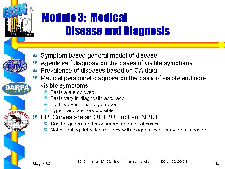
Module 3: Medical Disease and Diagnosis ¯ ¯ Symptom based general model of disease Agents self diagnose on the bases of visible symptoms Prevalence of diseases based on CA data Medical personnel diagnose on the basis of visible and nonvisible symptoms ¯ ¯ Tests are employed Tests vary in diagnostic accuracy Tests vary in time to get report Type 1 and 2 errors possible ¯ EPI Curves are an OUTPUT not an INPUT ¯ Can be generated for observed and actual cases ¯ Note: testing detection routines with diagnostics off may be misleading May 2003 © Kathleen M. Carley – Carnegie Mellon – ISRI, CASOS 35
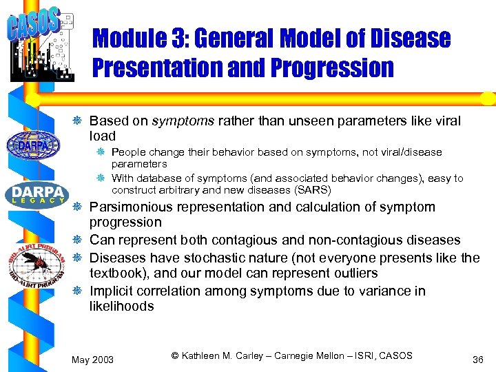
Module 3: General Model of Disease Presentation and Progression ¯ Based on symptoms rather than unseen parameters like viral load ¯ People change their behavior based on symptoms, not viral/disease parameters ¯ With database of symptoms (and associated behavior changes), easy to construct arbitrary and new diseases (SARS) ¯ Parsimonious representation and calculation of symptom progression ¯ Can represent both contagious and non-contagious diseases ¯ Diseases have stochastic nature (not everyone presents like the textbook), and our model can represent outliers ¯ Implicit correlation among symptoms due to variance in likelihoods May 2003 © Kathleen M. Carley – Carnegie Mellon – ISRI, CASOS 36
Module 3: Disease Characteristics ¯ Weaponized and Not ¯ Contagious and Not ¯ V 1/C 1 : 9 diseases; V 2/C 2 & C 3 : 60 diseases; V 2. 2/C 4/C 5: 70 diseases, desired – 600+ diseases ¯ Each disease has it’s own ¯ ¯ Set of symptoms Timing Variability in presentation based on age, gender, race Extent to which it is contagious ¯ Criteria for choosing the diseases for V 2 ¯ ¯ ¯ What diseases are required to be reported? What diseases are likely to be weaponized? What diseases are common – for adults, for children? What accounts for most ER visits? What diseases are most likely to be confused with the weaponized diseases? May 2003 © Kathleen M. Carley – Carnegie Mellon – ISRI, CASOS 37
Module 3: Disease Features ¯ Strain severity ¯ Onset locations ¯ A set of symptoms ¯ ¯ Evoking strength, P(D|S) (where D=disease, S=symptom) Frequency, P(S|D) Cost of treatment (low, medium, high) Visible or requiring test (tests are visible, low cost, high cost) ¯ Progression of disease within agent ¯ Infectious phase: agent has been infected but does not infect others ¯ Communicable phase: agent infects others (only exists for contagious diseases) ¯ Symptomatic phase: agent displays symptoms – Onset of specific symptoms is random ¯ Variations in onset and length of each phase in general – Known timing (CDC or JH web sites) – Additional variation per agent based on – Severity of strain – Agent age, gender, race, medical history – Treatment May 2003 © Kathleen M. Carley – Carnegie Mellon – ISRI, CASOS 38
Module 3: Model for Contagious Disease ¯ Transmission medium: contact, airborne, food, etc. ¯ When person comes into the contact with the transmission medium, disease transmission occurs with some probability. ¯ Planned - Persons have disease risk factors based on susceptibility, state of health, demographics. ¯ Phases: ¯ Infected: the length of time during which an bio-agent has entered the person’s body, the person has not displayed any symptom, and the person may or may not be infectious to others. ¯ Communicable: the length of time during which a person is infectious to others. The person may or may not display symptoms. This phase may overlap with infected & symptomatic phases. ¯ Symptomatic: the length of time during which a person shows symptoms. – to be divided into early and late. ¯ Modeled, at least partially, as non-deterministic automata. ¯ As past medical history affects the transition, this is a non-Markovian model. ¯ Any time within the duration of a state an intervention can occur, and the reality changes. ¯ The state of the disease can also affect the intervention, e. g, certain symptoms trigger certain behaviors. ¯ In contrast to SIR model, we model contagious diseases at the individual level and take intervention into account. May 2003 © Kathleen M. Carley – Carnegie Mellon – ISRI, CASOS 39
Module 3: List of Modeled Contagious Diseases Bacterial pharyngitis acute non streptococcal non gonoccocal, botulism, bubonic plague, campylobacter enteritis, cutaneous atypical mycobacterial infection, encephalitis acute viral, giardiasis intestinal, gram negative pneumonia non klebsiella, hepatitis A acute, herpes simplex encephalitis, immunice deficiency syndrome acquired (aids), infectious mononucleosis, influenza pneumonia, malaria, meningococcal meningitis, mycoplasma pneumonia, May 2003 plague meningitis, plague pneumonia, pneumococcla pneumonia, pulmonary legionellosis, salmonella enterocolitis non typhi, schistosomiasis systemic, shigellosis, staphylococcal pneumonia, staphylococcal scarlet fever toxic shock syndrome, streptococcal pharyngitis acute, streptococcus pyogenes pneumonia, syphilis primary, smallpox, tuberculosis chronic pulmonary, tuberculosis disseminated, varicella pneumonia, viral gastroenteritis, viral pharyngitis acute non herpetic © Kathleen M. Carley – Carnegie Mellon – ISRI, CASOS 40
Module 3: Model for Non-Contagious Disease ¯ Non-contagious disease do not have a communicable phase ¯ Some non-communicable can be spread by contact ¯ E. g. , anthrax spread by US Mail ¯ Implementation of this is planned ¯ Modeled, at least partially, as non-deterministic automata. ¯ Intervention affects how states in the model change ¯ E. g. , if anthrax infection is suspected to be present, this triggers the intervention such as giving Cipro antibiotics. Giving Cipro, in turn, ameliorates the possible symptoms and possibly cure the disease ¯ For weaponized diseases ¯ For short term non-contagious ¯ E. g. , food poisoning ¯ Outbreaks are randomly determined based on prevalence data ¯ For long term non-contagious diseases ¯ E. g. , angina, diabetes ¯ Given prevalence information initial population is “infected” – Subject to known race, gender, age distributions ¯ If Agent dies another agent at random is infected May 2003 © Kathleen M. Carley – Carnegie Mellon – ISRI, CASOS 41
Module 3: List of Modeled Non- Contagious Diseases Angina pectoris, anxiety neurosis, arteriolar nephrosclerosis benign essential hypertension, arteriosclerotic heart disease, bronchial asthma, bronchitis chronic simple, brucellosis, cardiogenic shock acute, chronic fatigue syndrome, cutaneous anthrax, depression, diabetes mellitus, disseminated intravascular coagulation, May 2003 fibromyalgia syndrome, heat exhaustion, hypertensive heart disease, hypovolemic shock, anthrax inhalational, myocardial infarction acute, obsessive compulsive neurosis, pulmonary emphysema, somatization disorder hysteria, staphylococcal gastroenteritis food poisoning, tension headache, tularemia menigitis © Kathleen M. Carley – Carnegie Mellon – ISRI, CASOS 42
Module 3: List of Modeled Weaponized Diseases ¯ Cutaneous Anthrax ¯ Inhalation Anthrax ¯ Smallpox ¯ Bubonic Plague May 2003 © Kathleen M. Carley – Carnegie Mellon – ISRI, CASOS 43
Module 3: Sources used in creating the disease database ¯ CDC ¯ Blue book ¯ Johns Hopkins ¯ Military textbook on chemical and biological warfare ¯ Kelly’s Textbook of Medicine ¯ Mendel’s Textbook of Infectious Diseases ¯ WHO report on Smallpox ¯ Medline ¯ Internist May 2003 © Kathleen M. Carley – Carnegie Mellon – ISRI, CASOS 44
Module 3: Medical Diagnosis “Institutionally Observed Diseases” ¯ Diagnosis of weaponized disease in Dr. and E. R. can be turned on or off ¯ Diagnosis occurs if agent goes to Dr. office or E. R. ¯ Diagnosis can be correct or not – both type 1 and 2 errors ¯ Diagnosis results in ¯ If at Dr. office – treatment or order test ¯ If at E. R. – treatment, test or admission to hospital ¯ Planned - Treatment may not be immediately effective ¯ Symptoms vary in whether they are visible or require a low or high cost test ¯ Diagnosis is done via inference ¯ In V 2 the inference model is based on the Columbia QMR model which uses evoking strengths to infer likelihood of various disease ¯ Differential diagnosis is possible corresponding to the onset symptoms ¯ Can handle agents with multiple diseases ¯ Each symptom has an evoking strength, P(D|S) (where D=disease, S=symptom) May 2003 © Kathleen M. Carley – Carnegie Mellon – ISRI, CASOS 45
Module 3: Tests for Diagnoses ¯ Diagnostic tests vary in ¯ Cost (not implemented yet) ¯ Time to get a result – 3 categories – Immediate (visible, immediate response, lowest cost) – Simple (quick response, low cost) – Complex (long response, high cost) ¯ Results from test impact: – Diagnosis – Intervention May 2003 © Kathleen M. Carley – Carnegie Mellon – ISRI, CASOS 46
Module 3: Diagnostic Latencies ¯ Dr. and ER diagnoses take a while to send reports ¯ Dr. report latency is based on: ¯ Data from Veridian ¯ ER report latency is based on: ¯ Data from Veridian ¯ Test latencies ¯ Range and mean is based on SME ¯ Specific latency randomly set given this range ¯ Planned – dynamically reduce latency when attack or major outbreak has been identified May 2003 © Kathleen M. Carley – Carnegie Mellon – ISRI, CASOS 47
Interventions ¯ Current ¯ When a disease is diagnosed in the simulated agent medication is provided ¯ With some probability, the agent then either recovers or dies immediately ¯ Plans ¯ C 4 ¯ Intervention takes a while to have an impact ¯ Range based on available data ¯ Depending on disease agent may remain able to infect others in this phase ¯ C 5 ¯ Intervention based on misdiagnosis has reduced or no ability to cure patient May 2003 © Kathleen M. Carley – Carnegie Mellon – ISRI, CASOS 48
Module 3: reporting EPI – curve data ¯ Actual Incidence – the number of new cases of the disease per day ¯ Actual Prevalence – the total number of the existing cases of the disease at this day ¯ Observed Incidence – the number of new cases of the disease diagnosed per day ¯ Observed Prevalence – the total number of the existing cases of the disease that have been diagnosed at this day Note – for weaponized diseases, if diagnosis is turned off observed incidence and prevalence will be 0 May 2003 © Kathleen M. Carley – Carnegie Mellon – ISRI, CASOS 49
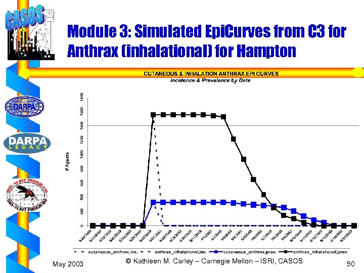
Module 3: Simulated Epi. Curves from C 3 for Anthrax (inhalational) for Hampton May 2003 © Kathleen M. Carley – Carnegie Mellon – ISRI, CASOS 50
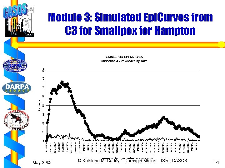
Module 3: Simulated Epi. Curves from C 3 for Smallpox for Hampton May 2003 © Kathleen M. Carley – Carnegie Mellon – ISRI, CASOS 51
Module 3: Planned Improvements ¯ Additional diseases ¯ E. g. , SARS ¯ Additional validation ¯ Separate each disease symptoms in to early and late ¯ Improved “background” and distractor diseases ¯ E. g. , accidents ¯ Link diagnosis to treatment ¯ Cost module for treatments ¯ Adjust treatment times based on capacity limits of Dr and E. R. to treat patients ¯ Adjust timing of symptoms to early/late presentation ¯ Improve generation module for initial population to populate with medical conditions whose timing is potentially greater than 2 years; e. g. , immuno compromised, angina, diabetes May 2003 © Kathleen M. Carley – Carnegie Mellon – ISRI, CASOS 52
Module 4: Agent Behavioral Model Characteristics of Simulated Agents ¯ Roles – father, teacher … ¯ Socio-demographic economic status ¯ Location ¯ Behaviors ¯ ¯ ¯ Interact – communicate, infect Recreate, school, work, sleep Seek treatment – OTC, Dr. E. R. (based on self. Diagnosis) Get medical info – phone, web Move (natural mobility) ¯ Ego net ¯ Natural biological time, e. g. , sleeping for 8 hours a day – every 4 hr or by day output ¯ Mental model of the disease May 2003 © Kathleen M. Carley – Carnegie Mellon – ISRI, CASOS 53
Module 4: Agent Interaction & Knowledge Process ¯ Build current social network: ¯ For each simulated agent that can interact, choose a random agent A from the agent’s ego net ¯ Compute the probabilities of interaction with A due to common knowledge P(K|I) and proximity P(D|I) ¯ Compute the probability of interaction P(I) as a weighted combination of P(K|I) and P(D|I): P(I) : = W, spatial* P(K|I) + (1 – W, spatial)*P(D|I) ¯ Throw a random die R : if R < P(I), then add A to the agent’s partner list ¯ Compute interaction effects: ¯ For each simulated agent, determine if the agent exchanges knowledge with each of its partners ¯ Update agent interaction timing info (used to determine if agent should interact each tick) May 2003 © Kathleen M. Carley – Carnegie Mellon – ISRI, CASOS 54
Module 4: Disease Exchange ¯ Disease exchanges: ¯ For each partner of a simulated agent (computed during the interaction step), throw a random die against the transmissivity of each communicable disease affecting the agent ¯ If the die roll fails and the partner does not already have the same disease instance (strain), infect the partner with the disease ¯ Do the same check for the agent for each communicable disease infecting the partner ¯ Planned – augment with agent susceptibility by sociodemographic category & medical history May 2003 © Kathleen M. Carley – Carnegie Mellon – ISRI, CASOS 55
Module 4: Entertainment ¯ Simulated agents may spend time on recreational activities ¯ Preferred entertainment is a function of ¯ ¯ ¯ Agent demographics Time of week/day Normal versus holiday/school vacation days Current health (varies by severity of illness) Planned – what friends are doing ¯ Entertainment types ¯ External (go to shopping mall, sports event, concert, restaurant) ¯ Home-based (read, watch TV, chat) ¯ Type of entertainment can affect likelihood of ¯ Being an attack victim ¯ Having knowledge about an attack May 2003 © Kathleen M. Carley – Carnegie Mellon – ISRI, CASOS 56
Module 4: Entertainment ¯ Bio. War C 2 entertainment support ¯ Support for external entertainment (e. g. restaurant dining, theaters, stadium events, shopping) ¯ Entertainment can override normal activities (e. g. skipping school to attend a concert) ¯ Bio. War C 3 enhancements ¯ Home-based events ¯ Stadium crowds ¯ Bio. War C 4 planned enhancements ¯ Prolonged recreation activities (longer than a single time tick) ¯ Entertainment interaction (e. g. disease knowledge is changed by online chatting) ¯ Agents can leave/enter simulation (e. g. vacation travel) May 2003 © Kathleen M. Carley – Carnegie Mellon – ISRI, CASOS 57
Module 4: Agents and Entertainment ¯ Two step determination process: 1. Does the simulated agent recreate this tick? 2. Where does recreation take place? ¯ Probability based, using actual time-use survey data: ¯ ¯ Season of year Generation (child of 18 or less versus adult) Gender Day of week ¯ Additional enhancements: ¯ Time of day ¯ Holidays (using the school_calendar package) May 2003 © Kathleen M. Carley – Carnegie Mellon – ISRI, CASOS 58
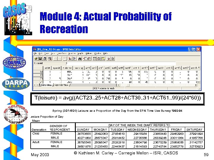
Module 4: Actual Probability of Recreation T(leisure) = avg((ACT 23. . 25+ACT 28+ACT 30. . 31+ACT 61. . 99)/(24*60)) Spring (3/21 -6/20) Leisure as a Proportion of the Day from the EPA Time Use Survey 1992 -94 Lesiure Proportion of Day Mean Generation Child Adult May 2003 GENDER OF RESPONDENT FEMALE SUNDAY. 38753655. 40271868. 36795546. 38601876 DAY OF THE WEEK THE DIARY REFERS TO MONDAY TUESDAY WEDNESDAY THURSDAY FRIDAY SATURDAY. 25492063. 27854610. 29415954. 23860480. 29462963. 37991898. 26675347. 25818452. 22735566. 26339286. 33011364. 41867766. 26096347. 25282818. 23604798. 23675259. 25868056. 31142757. 21235450. 22445437. 21614583. 22740784. 23852778. 32753923 © Kathleen M. Carley – Carnegie Mellon – ISRI, CASOS 59
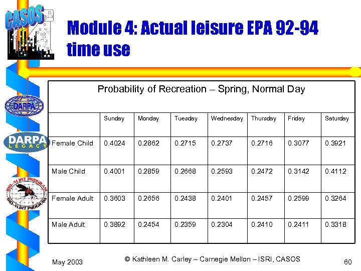
Module 4: Actual leisure EPA 92 -94 time use Probability of Recreation – Spring, Normal Day Sunday Monday Tuesday Wednesday Thursday Friday Saturday Female Child 0. 4024 0. 2862 0. 2715 0. 2737 0. 2716 0. 3077 0. 3921 Male Child 0. 4001 0. 2859 0. 2668 0. 2593 0. 2472 0. 3142 0. 4112 Female Adult 0. 3603 0. 2656 0. 2438 0. 2401 0. 2457 0. 2599 0. 3264 Male Adult 0. 3892 0. 2454 0. 2359 0. 2304 0. 2410 0. 2411 0. 3318 May 2003 © Kathleen M. Carley – Carnegie Mellon – ISRI, CASOS 60
Module 4: Validation and Tuning of Entertainment ¯ Primary data source: EPA Time Use survey (1994) – access to raw data ¯ Two critical data types: ¯ Time spent by activity category ¯ Time spent in locations ¯ Must infer certain critical values: ¯ Time spent in recreation at specific locations ¯ Holidays ¯ Time of day variations ¯ Bio. War Validated for: ¯ Annual recreation rates ¯ School absenteeism rates May 2003 © Kathleen M. Carley – Carnegie Mellon – ISRI, CASOS 61
Module 4: School Absenteeism ¯ Simulated agents are absent from school due to: ¯ Illness ¯ Skipping ¯ Other ¯ Probability of non illness absence set by school level ¯ Actual data from NCES Indicator 17 & Indicator 42 -1 ¯ Actual data from Veridian ¯ Non illness absence determined randomly ¯ Minor exceptions ¯ Higher absenteeism prior to and after weekend holiday ¯ No school on weekends, summer, holidays ¯ Planned ¯ Reason for absenteeism to impact interaction May 2003 © Kathleen M. Carley – Carnegie Mellon – ISRI, CASOS 62
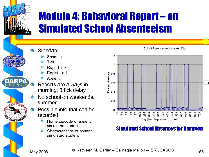
Module 4: Behavioral Report – on Simulated School Absenteeism ¯ Standard ¯ ¯ ¯ School id Tick Report tick Registered Absent ¯ Reports are always in morning, 3 tick delay ¯ No school on weekends, summer ¯ Possible info that can be recorded ¯ Home zipcode of absent simulated student ¯ Characteristics of absent simulated student May 2003 Simulated School Absences for Hampton © Kathleen M. Carley – Carnegie Mellon – ISRI, CASOS 63
Module 4: Work Site Behavior ¯ Simulated agents are absent from work due to: ¯ Illness ¯ Other ¯ Actual Data from Veridian ¯ Non illness absence determined randomly at pre-specified level using Veridian Data ¯ Minor exception ¯ Higher absenteeism prior to and after weekend holiday ¯ No work on major holidays or weekends ¯ Phone calls ¯ Data from IBM ¯ Web visits ¯ Data from on-line hit rate for medical sites ¯ Planned ¯ Health survey ¯ Outgoing web hits and email May 2003 © Kathleen M. Carley – Carnegie Mellon – ISRI, CASOS 64
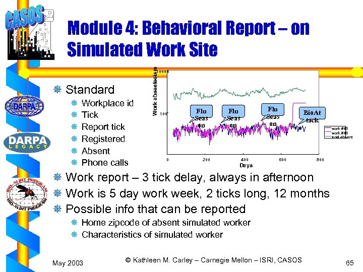
Work absenteeism Module 4: Behavioral Report – on Simulated Work Site 10000 ¯ Standard ¯ ¯ ¯ Workplace id Tick Report tick Registered Absent Phone calls 100 0 Flu Seas on 200 Flu Seas on 400 600 Bio. At tack work #45 work #46 total absent 800 Days ¯ Work report – 3 tick delay, always in afternoon ¯ Work is 5 day work week, 2 ticks long, 12 months ¯ Possible info that can be reported ¯ Home zipcode of absent simulated worker ¯ Characteristics of simulated worker May 2003 © Kathleen M. Carley – Carnegie Mellon – ISRI, CASOS 65
Module 4: Seeking Treatment ¯ Propensity to seek treatment affected by ¯ ¯ Socio-demographic position (age, race, gender) Socio-economic status Severity of visible symptoms Planned – by medical history ¯ Type of treatment also impacted by availability ¯ E. g. can’t go to pharmacy or Dr. if closed ¯ Reporting delays ¯ Based on SME estimates and IBM data May 2003 © Kathleen M. Carley – Carnegie Mellon – ISRI, CASOS 66
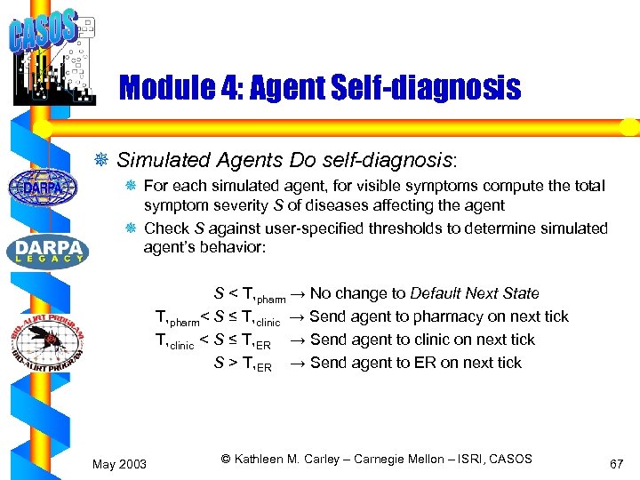
Module 4: Agent Self-diagnosis ¯ Simulated Agents Do self-diagnosis: ¯ For each simulated agent, for visible symptoms compute the total symptom severity S of diseases affecting the agent ¯ Check S against user-specified thresholds to determine simulated agent’s behavior: S < T, pharm → No change to Default Next State T, pharm< S ≤ T, clinic → Send agent to pharmacy on next tick T, clinic < S ≤ T, ER → Send agent to clinic on next tick S > T, ER → Send agent to ER on next tick May 2003 © Kathleen M. Carley – Carnegie Mellon – ISRI, CASOS 67
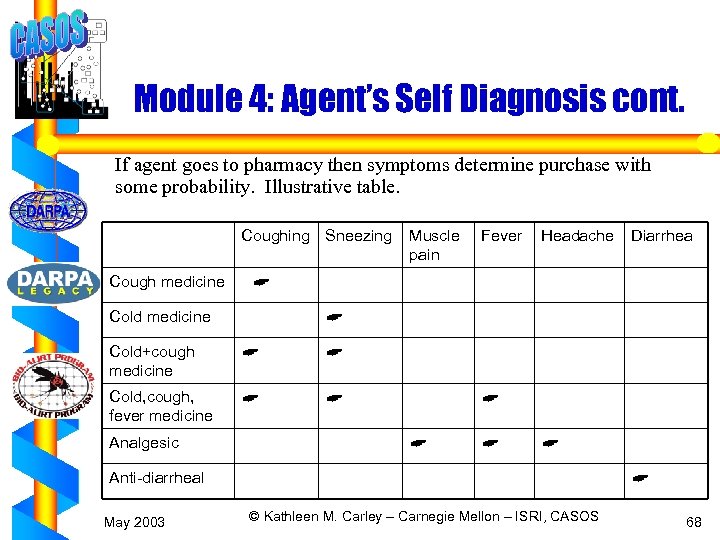
Module 4: Agent’s Self Diagnosis cont. If agent goes to pharmacy then symptoms determine purchase with some probability. Illustrative table. Coughing Sneezing Cough medicine Muscle pain Fever Headache Diarrhea A Cold medicine A Cold+cough medicine A A Cold, cough, fever medicine A A Analgesic A A Anti-diarrheal May 2003 A © Kathleen M. Carley – Carnegie Mellon – ISRI, CASOS 68
Module 4: Pharmacy Behavior ¯ Simulated agents go to the pharmacy nearest work if at work or nearest home if at home ¯ Simulated agents purchase a “unit” of an item ¯ Items are assumed to be one week supply ¯ Children under 12 not allowed to purchase ¯ Planned: ¯ ¯ Purchasing for others Additional items to be purchased Variation in purchased amount (supply), multiple purchases Purchasing increases in December May 2003 © Kathleen M. Carley – Carnegie Mellon – ISRI, CASOS 69
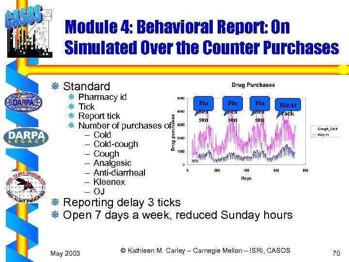
Module 4: Behavioral Report: On Simulated Over the Counter Purchases ¯ Standard ¯ ¯ Pharmacy id Tick Report tick Number of purchases of – Cold-cough – Cough – Analgesic – Anti-diarrheal – Kleenex – OJ Flu Sea son Bio. At tack ¯ Reporting delay 3 ticks ¯ Open 7 days a week, reduced Sunday hours May 2003 © Kathleen M. Carley – Carnegie Mellon – ISRI, CASOS 70
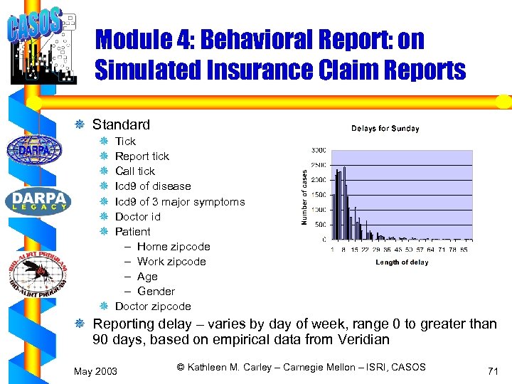
Module 4: Behavioral Report: on Simulated Insurance Claim Reports ¯ Standard ¯ ¯ ¯ ¯ Tick Report tick Call tick Icd 9 of disease Icd 9 of 3 major symptoms Doctor id Patient – Home zipcode – Work zipcode – Age – Gender ¯ Doctor zipcode ¯ Reporting delay – varies by day of week, range 0 to greater than 90 days, based on empirical data from Veridian May 2003 © Kathleen M. Carley – Carnegie Mellon – ISRI, CASOS 71
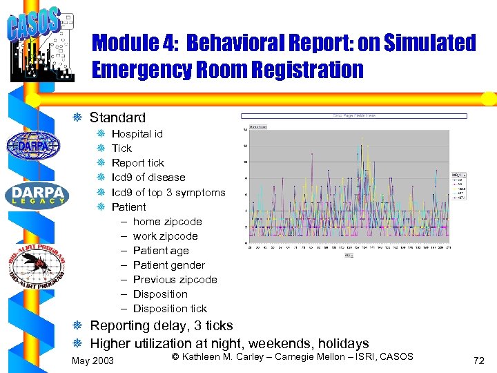
Module 4: Behavioral Report: on Simulated Emergency Room Registration ¯ Standard ¯ ¯ ¯ Hospital id Tick Report tick Icd 9 of disease Icd 9 of top 3 symptoms Patient – home zipcode – work zipcode – Patient age – Patient gender – Previous zipcode – Disposition tick ¯ Reporting delay, 3 ticks ¯ Higher utilization at night, weekends, holidays May 2003 © Kathleen M. Carley – Carnegie Mellon – ISRI, CASOS 72
Module 4: Additional Plans ¯ Social influence on behavior ¯ Behavior for others ¯ E. g. , Parent’s purchasing OTC based on child’s symptoms ¯ ¯ ¯ Improved web and phone call behavior from home/work Appropriate scaling of interaction Survey answering behavior Possible panic module Automate results collection and comparison. Comparison against other data sources: ¯ Poll results ¯ Other time-use data sets ¯ Additional behavioral data May 2003 © Kathleen M. Carley – Carnegie Mellon – ISRI, CASOS 73
Module 5: Geometry ¯ Conversion between ¯ ZCTA – UTM – Lat/Lon ¯ Linkage of ZCTA to USPS ¯ All agents/locations have location ¯ Assorted pre and post-processors ¯ Location impacts choice of E. R. , Dr. Pharmacy … ¯ Plan – link to Arcview May 2003 © Kathleen M. Carley – Carnegie Mellon – ISRI, CASOS 74
Geometry In Bio. War ¯ Census cartographic boundaries enclose simulation area – polygon vertices specified by longitude/latitude ¯ Positions of locations, agents, outbreaks, and attacks specified by longitude/latitude ¯ Most distances computed in longitude/latitude ¯ Outdoor attack position, agent positions dynamically converted into UTM coordinates to compute distances from attack ¯ Geometry composed of several simple classes May 2003 © Kathleen M. Carley – Carnegie Mellon – ISRI, CASOS 75
Geometry In Bio. War (Cont’d) – Objects ¯ Points ¯ Longitude/latitude and UTM coordinate systems ¯ Conversion between systems using several ellipsoid definitions ¯ Polygons ¯ Generically programmed vertex positions (can use longitude/latitude, UTM, etc. ) ¯ Several geometric operations (e. g. point containment) ¯ Census tracts ¯ Polygons with Census-assigned attributes ¯ Currently handles school districts, ZCTA’s, block groups, and census tracts ¯ Future integration with Census Tiger/Line to improve e. g. agent distribution over census tracts May 2003 © Kathleen M. Carley – Carnegie Mellon – ISRI, CASOS 76
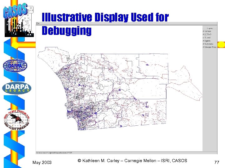
Illustrative Display Used for Debugging May 2003 © Kathleen M. Carley – Carnegie Mellon – ISRI, CASOS 77
Module 6: Weather ¯ Weather module includes wind and climate ¯ Added and validated for C 2 ¯ Provides distinct wind and weather patterns for each city ¯ Linked to dispersion via aerosolized attacks ¯ Planned Improvement – link to HPAC ¯ Would enable improved reporting capabilities ¯ Would enable faster modeling of alternative cities ¯ Would enable forecasting on current data May 2003 © Kathleen M. Carley – Carnegie Mellon – ISRI, CASOS 78
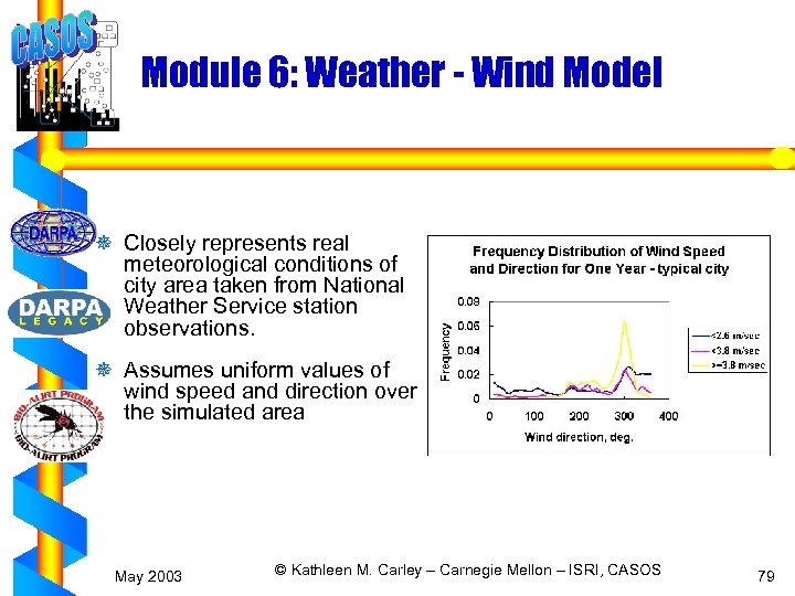
Module 6: Weather - Wind Model ¯ Closely represents real meteorological conditions of city area taken from National Weather Service station observations. ¯ Assumes uniform values of wind speed and direction over the simulated area May 2003 © Kathleen M. Carley – Carnegie Mellon – ISRI, CASOS 79
Module 6: Wind Model Limitations ¯ Wind Model does not address ¯ Terrain height ¯ Building wake ¯ Seasonal differences ¯ Wind direction changes by at most one sector from one tick to the next May 2003 © Kathleen M. Carley – Carnegie Mellon – ISRI, CASOS 80
Module 6: What varies for wind and what impacts it Wind characteristics: ¯ Wind direction is the direction from which the wind comes ¯ Speed Meteorology impacts wind ¯ Pasquill atmospheric stability class ¯ Temperature ¯ Mixing height Current Wind Model assumes moderate insulation and thinly overcast cloud conditions. May 2003 © Kathleen M. Carley – Carnegie Mellon – ISRI, CASOS 81

Module 6: Sources of Data for Wind Model ¯ Empirical data – www. epa. gov/scram 001/ ¯ Rod Barratt “Atmospheric Dispersion Modeling” ¯ D. Bruce Turner “Workbook of Atmospheric Dispersion Estimates” ¯ Meselson, Matthew “Note Regarding Source Strength”, ASA Newsletter, article 01 -6 a (www. asanltr. com). May 2003 © Kathleen M. Carley – Carnegie Mellon – ISRI, CASOS 82
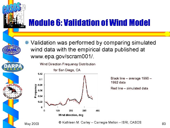
Module 6: Validation of Wind Model ¯ Validation was performed by comparing simulated wind data with the empirical data published at www. epa. gov/scram 001/. Wind Direction Frequency Distribution for San Diego, CA Black line – average 1990 – 1992 data Red line – simulated data May 2003 © Kathleen M. Carley – Carnegie Mellon – ISRI, CASOS 83
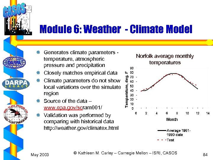
Module 6: Weather - Climate Model ¯ Generates climate parameters temperature, atmospheric pressure and precipitation ¯ Closely matches empirical data ¯ Climate parameters do not show local variations over the simulated region ¯ Source of the data – www. epa. gov/scram 001/ ¯ Validation was performed by comparing with historical data http: //weather. gov/climatex. html May 2003 Norfolk average monthly temperatures © Kathleen M. Carley – Carnegie Mellon – ISRI, CASOS 84
Module 7: Dispersion module for Aerosolized Attack ¯ Inputs: Emission information - location of the source and height of the release; Meteorological parameters – Pasquill stability class, wind direction, wind speed ¯ Outputs: Dosage inhaled by the agent ¯ Module uses modified Gaussian Puff Equation to estimate total dosage from finite release. ¯ Described in geographical coordinate system (lat/lon) which is transformed to/from UTM coordinate system and local coordinate system with the origin at the bio-release point. May 2003 © Kathleen M. Carley – Carnegie Mellon – ISRI, CASOS 85
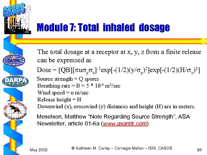
Module 7: Total inhaled dosage The total dosage at a receptor at x, y, z from a finite release can be expressed as Dose = [QB][pusysz]-1 exp[-(1/2)(y/sy)2]exp[-(1/2)(H/sz)2] Source strength = Q spores Breathing rate = B = 5 * 10 -4 m 3/sec Wind speed = u m/sec Release height = H Downwind (x), crosswind (y) distances and height (H) are in meters. Meselson, Matthew “Note Regarding Source Strength”, ASA Newsletter, article 01 -6 a (www. asanltr. com). May 2003 © Kathleen M. Carley – Carnegie Mellon – ISRI, CASOS 86
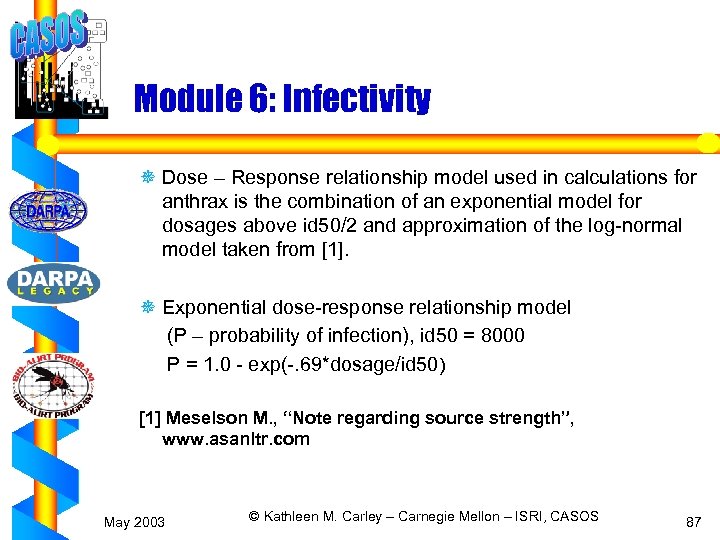
Module 6: Infectivity ¯ Dose – Response relationship model used in calculations for anthrax is the combination of an exponential model for dosages above id 50/2 and approximation of the log-normal model taken from [1]. ¯ Exponential dose-response relationship model (P – probability of infection), id 50 = 8000 P = 1. 0 - exp(-. 69*dosage/id 50) [1] Meselson M. , “Note regarding source strength”, www. asanltr. com May 2003 © Kathleen M. Carley – Carnegie Mellon – ISRI, CASOS 87
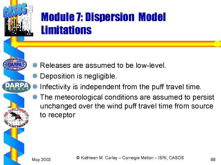
Module 7: Dispersion Model Limitations ¯ Releases are assumed to be low-level. ¯ Deposition is negligible. ¯ Infectivity is independent from the puff travel time. ¯ The meteorological conditions are assumed to persist unchanged over the wind puff travel time from source to receptor May 2003 © Kathleen M. Carley – Carnegie Mellon – ISRI, CASOS 88
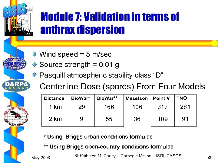
Module 7: Validation in terms of anthrax dispersion ¯ Wind speed = 5 m/sec ¯ Source strength = 0. 01 g ¯ Pasquill atmospheric stability class “D” Centerline Dose (spores) From Four Models Distance Bio. War* 1 km 29 2 km 9 Bio. War** Meselson Point V TNO 166 106 317 281 55 36 109 91 * Using Briggs urban conditions formulae ** Using Briggs open-country conditions formulae May 2003 © Kathleen M. Carley – Carnegie Mellon – ISRI, CASOS 89
Module 7: Source of data for validation ¯ Meselson, Matthew “Note Regarding Source Strength”, ASA Newsletter, article 01 -6 a ¯ POINT V – “Methodology for Chemical Hazard Prediction”, DOD, 1980, p. 17 ¯ TNO – TNO Defense Research, Rijswijk, The Netherlands ¯ Possible reasons for the discrepancy: - Bio. War uses Briggs dispersion parameters formulae for urban conditions while sources above uses formulae for open-country conditions - Military methodologies tend to overestimate the effect in order to protect troops May 2003 © Kathleen M. Carley – Carnegie Mellon – ISRI, CASOS 90
Module 8: Attack Scenario Module ¯ Attacks are created following the scenarios ¯ Attack scenario allows maximum flexibility ¯ Attacks vary based on ¯ ¯ ¯ Locations Inside or outside of building Date Time of Day Agent – Carrier – Airborne (contagion and non-contagion module), waterborne, foodborne, other – Non-airborne not done – Severity – Pathogen (weaponized disease) May 2003 © Kathleen M. Carley – Carnegie Mellon – ISRI, CASOS 91
Module 8: Attack Parameters ¯ Land or airborne attack type ¯ Spray or explosion type (by selecting release efficiency) ¯ Specification: – Pathogen – Biomaterial mass, release height and efficiency – Random or fixed time/date – Random or fixed locations – Single point or multi-point – Impact (low, medium, high based on number of people actually affected) May 2003 © Kathleen M. Carley – Carnegie Mellon – ISRI, CASOS 92
Module 8: Attack Scenario Examples ¯ Generate a medium, single-point spray attack between 100 and 200 ticks at an altitude of 20 m, using 1. 25 kg of material for an attack at 5% efficiency. - out medium anthrax_inhalational 100 200 1. 25 kg. 05 20 m ; ¯ Generate a large, multi-point airborne attack at 22: 00 on July 4, 2002 an altitude of 300 m, using 25 kg of material for an attack at 10% efficiency. Distribute 7 bombs along an attack line of 1. 5 km - out large anthrax_inhalational 2002/7/4 22: 00 25 kg. 1 300 m 1. 5 km 7 ; May 2003 © Kathleen M. Carley – Carnegie Mellon – ISRI, CASOS 93
May 2003 © Kathleen M. Carley – Carnegie Mellon – ISRI, CASOS 94
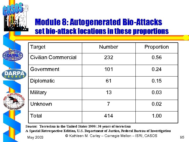
Module 8: Autogenerated Bio-Attacks set bio-attack locations in these proportions Target Number Proportion Civilian Commercial 232 0. 56 Government 101 0. 24 Diplomatic 61 0. 15 Military 13 0. 03 Unknown 7 0. 02 414 1. 00 Total Source: Terrorism in the United States 1999: 30 years of terrorism A Special Retrospective Edition, U. S. Department of Justice, Federal Bureau of Investigation © Kathleen M. Carley – Carnegie Mellon – ISRI, CASOS May 2003 95
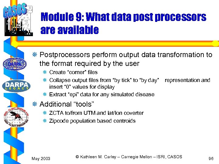
Module 9: What data post processors are available ¯ Postprocessors perform output data transformation to the format required by the user ¯ Create “corner” files ¯ Collapse output files from “by tick” to “by day” insert “ 0” values for display ¯ Extract “epi” data for any simulated disease representation and ¯ Additional “tools” ¯ ZCTA to/from UTM and lat/lon coverter ¯ Zipcode population based centroids May 2003 © Kathleen M. Carley – Carnegie Mellon – ISRI, CASOS 96
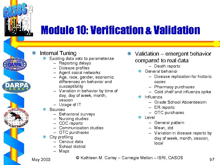
Module 10: Verification & Validation ¯ Internal Tuning ¯ Existing data sets to parameterize – Reporting delays – Disease profiles – Agent social networks – Age, race, gender, economic differences on behavior and susceptibility – Variation in behavior by time of day, day of week, month, season – Usage of IT ¯ Sources – Behavioral surveys – Nursing studies – CDC reports – Communication studies – OTC purchases ¯ City profiling – Census data – School district – Maps May 2003 ¯ Validation – emergent behavior compared to real data – Death reports ¯ General behavior – Disease replication for historic cases – Pharmacy purchases – Cold shelf and influenza spike ¯ Influenza – Grade School Absenteeism – ER reports – OTC purchases ¯ Level – General pattern – Mean, std – Variation in disease reports by day of week, month, season, local © Kathleen M. Carley – Carnegie Mellon – ISRI, CASOS 97
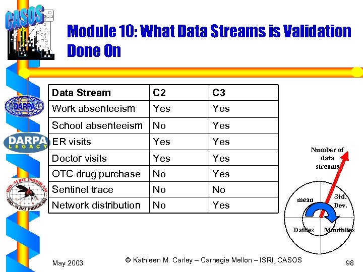
Module 10: What Data Streams is Validation Done On Data Stream C 2 C 3 Work absenteeism Yes School absenteeism No Yes ER visits Yes Doctor visits Yes OTC drug purchase No Yes Sentinel trace No No Number of data streams May 2003 No Yes Std. Dev. Dailies Network distribution mean Monthlies © Kathleen M. Carley – Carnegie Mellon – ISRI, CASOS 98
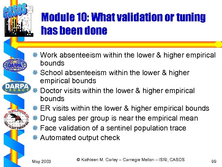
Module 10: What validation or tuning has been done ¯ Work absenteeism within the lower & higher empirical bounds ¯ School absenteeism within the lower & higher empirical bounds ¯ Doctor visits within the lower & higher empirical bounds ¯ ER visits within the lower & higher empirical bounds ¯ Drug sales per group is near the empirical mean ¯ Face validation of a sentinel population trace ¯ Automated output check May 2003 © Kathleen M. Carley – Carnegie Mellon – ISRI, CASOS 99
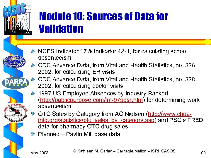
Module 10: Sources of Data for Validation ¯ NCES Indicator 17 & Indicator 42 -1, for calculating school absenteeism ¯ CDC Advance Data, from Vital and Health Statistics, no. 326, 2002, for calculating ER visits ¯ CDC Advance Data, from Vital and Health Statistics, no. 328, 2002, for calculating doctor visits ¯ 1997 US Employee Absences by Industry Ranked (http: //publicpurpose. com/lm-97 absr. htm) for determining work absenteeism ¯ OTC Sales by Category from AC Nielsen (http: //www. chpainfo. org/statistics/otc_sales_by_category. asp) and PSC’s FRED data for pharmacy OTC drug sales ¯ Planned – Pavlin Mil. base data May 2003 © Kathleen M. Carley – Carnegie Mellon – ISRI, CASOS 100
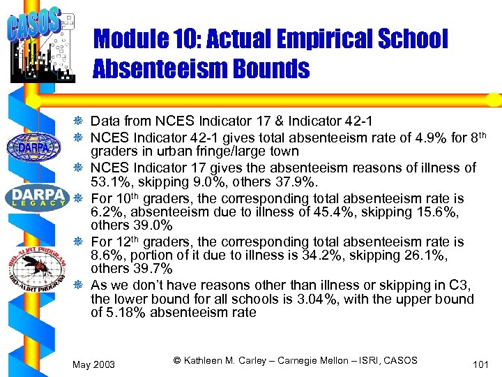
Module 10: Actual Empirical School Absenteeism Bounds ¯ Data from NCES Indicator 17 & Indicator 42 -1 ¯ NCES Indicator 42 -1 gives total absenteeism rate of 4. 9% for 8 th graders in urban fringe/large town ¯ NCES Indicator 17 gives the absenteeism reasons of illness of 53. 1%, skipping 9. 0%, others 37. 9%. ¯ For 10 th graders, the corresponding total absenteeism rate is 6. 2%, absenteeism due to illness of 45. 4%, skipping 15. 6%, others 39. 0% ¯ For 12 th graders, the corresponding total absenteeism rate is 8. 6%, portion of it due to illness is 34. 2%, skipping 26. 1%, others 39. 7% ¯ As we don’t have reasons other than illness or skipping in C 3, the lower bound for all schools is 3. 04%, with the upper bound of 5. 18% absenteeism rate May 2003 © Kathleen M. Carley – Carnegie Mellon – ISRI, CASOS 101
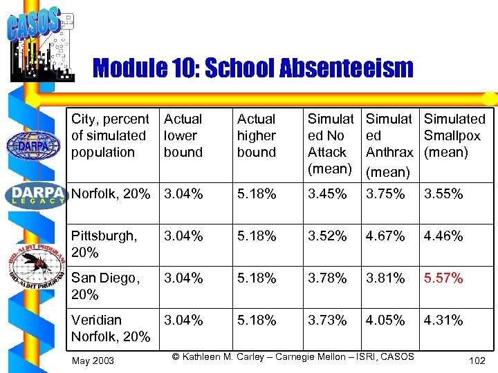
Module 10: School Absenteeism City, percent of simulated population Actual lower bound Actual higher bound Simulat ed No Attack (mean) Simulated ed Smallpox Anthrax (mean) Norfolk, 20% 3. 04% 5. 18% 3. 45% 3. 75% 3. 55% Pittsburgh, 20% 3. 04% 5. 18% 3. 52% 4. 67% 4. 46% San Diego, 20% 3. 04% 5. 18% 3. 78% 3. 81% 5. 57% Veridian 3. 04% Norfolk, 20% 5. 18% 3. 73% 4. 05% 4. 31% May 2003 © Kathleen M. Carley – Carnegie Mellon – ISRI, CASOS 102
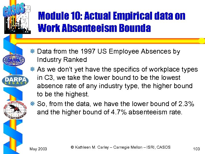
Module 10: Actual Empirical data on Work Absenteeism Bounda ¯ Data from the 1997 US Employee Absences by Industry Ranked ¯ As we don’t yet have the specifics of workplace types in C 3, we take the lower bound to be the lowest absence rate of any industry type, the higher bound to be the highest. ¯ So, from the data, we have the lower bound of 2. 3% and the higher bound of 4. 7% absenteeism rate. May 2003 © Kathleen M. Carley – Carnegie Mellon – ISRI, CASOS 103
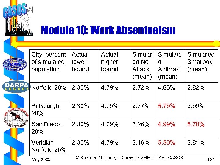
Module 10: Work Absenteeism City, percent Actual of simulated lower population bound Actual higher bound Simulat ed No Attack (mean) Simulated d Smallpox Anthrax (mean) Norfolk, 20% 2. 30% 4. 79% 2. 72% 4. 65% 2. 82% Pittsburgh, 20% 2. 30% 4. 79% 2. 77% 5. 79% 3. 99% San Diego, 20% 2. 30% 4. 79% 3. 26% 4. 99% 5. 78% Veridian 2. 30% Norfolk, 20% 4. 79% 3. 16% 5. 50% 3. 81% May 2003 © Kathleen M. Carley – Carnegie Mellon – ISRI, CASOS 104
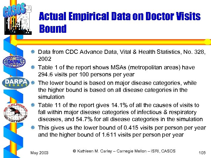
Actual Empirical Data on Doctor Visits Bound ¯ Data from CDC Advance Data, Vital & Health Statistics, No. 328, 2002 ¯ Table 1 of the report shows MSAs (metropolitan areas) have 294. 6 visits per 100 persons per year ¯ The lower bound is based on major disease categories, while the higher bound is based on all disease categories in the simulation ¯ Table 11 of the report gives 14. 1% of all the causes of visits to fall within major disease categories of infectious & respiratory diseases, and 54. 7% for all disease categories in the simulation ¯ This gives us the lower bound of 0. 415 visits person per year and the higher bound of 1. 611 visits person per year May 2003 © Kathleen M. Carley – Carnegie Mellon – ISRI, CASOS 105
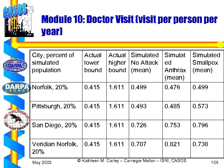
Module 10: Doctor Visit (visit person per year) City, percent of simulated population Actual lower bound Actual Simulated Simulat higher No Attack ed bound (mean) Anthrax (mean) Simulated Smallpox (mean) Norfolk, 20% 0. 415 1. 611 0. 499 0. 476 0. 499 Pittsburgh, 20% 0. 415 1. 611 0. 493 0. 485 0. 573 San Diego, 20% 0. 415 1. 611 0. 726 0. 753 0. 796 Veridian Norfolk, 20% 0. 415 1. 611 0. 707 0. 821 0. 738 May 2003 © Kathleen M. Carley – Carnegie Mellon – ISRI, CASOS 106
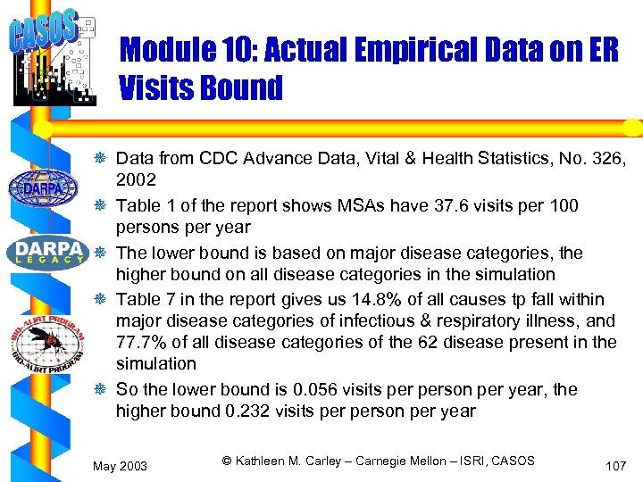
Module 10: Actual Empirical Data on ER Visits Bound ¯ Data from CDC Advance Data, Vital & Health Statistics, No. 326, 2002 ¯ Table 1 of the report shows MSAs have 37. 6 visits per 100 persons per year ¯ The lower bound is based on major disease categories, the higher bound on all disease categories in the simulation ¯ Table 7 in the report gives us 14. 8% of all causes tp fall within major disease categories of infectious & respiratory illness, and 77. 7% of all disease categories of the 62 disease present in the simulation ¯ So the lower bound is 0. 056 visits person per year, the higher bound 0. 232 visits person per year May 2003 © Kathleen M. Carley – Carnegie Mellon – ISRI, CASOS 107
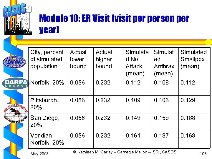
Module 10: ER Visit (visit person per year) City, percent of simulated population Actual lower bound Actual higher bound Simulate d No Attack (mean) Simulat ed Anthrax (mean) Simulated Smallpox (mean) Norfolk, 20% 0. 056 0. 232 0. 112 0. 108 0. 112 Pittsburgh, 20% 0. 056 0. 232 0. 109 0. 106 0. 129 San Diego, 20% 0. 056 0. 232 0. 149 0. 159 0. 188 Veridian Norfolk, 20% 0. 056 0. 232 0. 161 0. 187 0. 168 May 2003 © Kathleen M. Carley – Carnegie Mellon – ISRI, CASOS 108
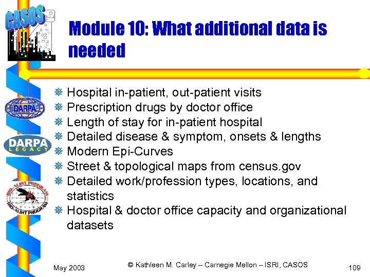
Module 10: What additional data is needed ¯ Hospital in-patient, out-patient visits ¯ Prescription drugs by doctor office ¯ Length of stay for in-patient hospital ¯ Detailed disease & symptom, onsets & lengths ¯ Modern Epi-Curves ¯ Street & topological maps from census. gov ¯ Detailed work/profession types, locations, and statistics ¯ Hospital & doctor office capacity and organizational datasets May 2003 © Kathleen M. Carley – Carnegie Mellon – ISRI, CASOS 109
Module 10: What additional validation or tuning is planned ¯ ¯ ¯ Std. Dev. , monthlies, and dailies for all streams Pharmacy visits In-patient & out-patient visits Hospital visits, in contrast to ER visits Weekday & monthly variation of drug purchase based on FRED data ¯ Identifying the variability of parameters & model variables ¯ Validation against Pavlin Mil. Base data ¯ Extending WIZER automated output check to tune input & model parameters May 2003 © Kathleen M. Carley – Carnegie Mellon – ISRI, CASOS 110
Module 10: Extended Validation Plan ¯ Additional utilization by other groups ¯ For current output variables ¯ Show validity for Std. Dev. , monthly differences, daily differences ¯ Locate additional data sources ¯ Do comparison with Pavlin data May 2003 © Kathleen M. Carley – Carnegie Mellon – ISRI, CASOS 111
Extended capability analysis ¯ By Sept 1 ¯ Detailed comparison of predictions compared to Standard SIR for: ¯ Small pox ¯ Inhalational Anthrax ¯ Cutaneous Anthrax May 2003 © Kathleen M. Carley – Carnegie Mellon – ISRI, CASOS 112
Wizer: The need for automated analysis and validation ¯ Validation is difficult to do manually due to model complexity - the significant number of input and model parameters, output variables ¯ Scaling Bio. War up to take in more models – local models and diverse secondary data streams – would increase the code size and thus the need for validation and test for reliability ¯ Insufficient testing is a problem ¯ An automated tool that analyzes software and rates its reliability by examining the response surface relative to empirical data is needed May 2003 © Kathleen M. Carley – Carnegie Mellon – ISRI, CASOS 113
Wizer Extends Response Surface Methods ¯ Response surface methodology: ¯ collection of mathematical and statistical techniques for the modeling & analysis of problems in which a response of interest is influenced by several variables and the objective this response. ¯ Bio. War has a complex response surface. ¯ Putting Bio. War in Spec can be viewed as a multi-dimensional numeric & symbolic optimization problem ¯ E. g. , school absenteeism is influenced by student health status, skipping, or other reasons such as school district announcements. ¯ Within these symbolic variables, there are numeric values to denote the probability, the trends, etc. ¯ Wizer ¯ extends response surface methodology by performing knowledge-intensive search steps via a social inference engine ¯ instead of doing conventional mathematical & statistical calculations ¯ Better faster validation ¯ Better faster tuning May 2003 © Kathleen M. Carley – Carnegie Mellon – ISRI, CASOS 114
Wizer: Version 0 Implementation ¯ Automated system for What if Analysis and Validation: ¯ [Version 0, Implemented & deployed in C 3: ] Takes the simulated output data and the set of validation specs and "sets off an alarm" if ¯ When the distribution is known – if the simulated data is ever more than 1 std-dev away from the spec ¯ When the distribution is not known – if the simulated data is outside the allowable range on the spec ¯ Automated search for set of changes to move the simulation back within spec. To do this, Wizer utilizes social, epidemiological, geographical, etc. knowledge via inference engine. Wizer can be viewed as an intelligent search step generator. ¯ Note: user is able to specify to this system how mutable the input parameters are ¯ for some parameters you can vary over a wide range while other parameters are fixed ¯ how mutable would depend on the quality of the data underlying them May 2003 © Kathleen M. Carley – Carnegie Mellon – ISRI, CASOS 115
Wizer: Planned Roadmap ¯ Adding knowledge base of social & epidemiological expertise ¯ Building an inference engine on top of knowledge base ¯ Interfacing the inference engine with Bio. War simulation ¯ Adding meta-modeler ¯ Adding experiment designer ¯ Performing the 1 st fully automated test run of automated validation of Bio. War using Wizer May 2003 © Kathleen M. Carley – Carnegie Mellon – ISRI, CASOS 116
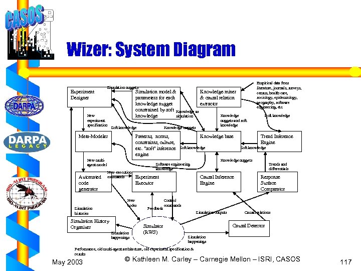
Wizer: System Diagram Experiment Designer New experiment specification Simulation model & Knowledge miner parameters for each & causal relation knowledge nugget extractor constrained by soft Knowledge as Knowledge simulation knowledge Patterns, norms, constraints, culture, etc. “soft” inference engine New multiagent model New execution commands Simulation histories Simulation History Organizer Simulation happenings Knowledge base Soft knowledge Experiment Executor Feedback Simulator (RWS) Trend Inference Engine Soft knowledge Knowledge nuggets Software engineering knowledge New codes Soft knowledge nuggets and soft knowledge Knowledge nuggets Soft knowledge Meta-Modeler Automated code generator Empirical data from literature, journals, surveys, census, health care, sociology, epidemiology, geography, software engineering, etc. Simulation nuggets Causal Inference Engine Trends and differentials Response Surface Comparator Control commands Simulation outputs Causal relations Causal Detector Simulation happenings Performance, old multi-agent architecture, old experiment specification & results May 2003 © Kathleen M. Carley – Carnegie Mellon – ISRI, CASOS 117
What were major changes going from C 1 to C 2 ¯ ¯ New wind & climate models New ego networks New entertainment locations Scaled empirical data for locations (of schools, doctor office, & ERs) ¯ Increase from ¯ ¯ 10 to 60 diseases 27 K to 260 K agents 5 to 10 OTC purchases 100 to 1000 Locations ¯ New metro areas – Norfolk, Hampton ¯ True locations for schools May 2003 © Kathleen M. Carley – Carnegie Mellon – ISRI, CASOS 118
What were major changes going from C 2 to C 3 (one month timeframe) ¯ Increase from ¯ 260 K to 560 K agents ¯ 1 K to 10 K locations ¯ True lat/lon for all non-work locations ¯ Avg. school absenteeism and pharmacy drug sales validated ¯ Automated output check (WIZER version 0) implemented and deployed ¯ Improved social networks, family units created ¯ Climate precipitation module ¯ Validated social network distributions ¯ Speeded up city and network generation ¯ Multi-threaded code, the 1 st step of parallelization, capable of utilizing multiple processors at once May 2003 © Kathleen M. Carley – Carnegie Mellon – ISRI, CASOS 119
Planned Improvements for C 4 ¯ Adding in-patient hospital stay ¯ Refining diagnosis and treatment modules ¯ Refined non-contagious disease mode ¯ Increased optimization ¯ Occupational types ¯ Validation with existing data at Std. Dev. & where possible monthly and daily differences May 2003 © Kathleen M. Carley – Carnegie Mellon – ISRI, CASOS 120
Planned Improvements for C 5 ¯ Additional cities – San Fancisco, DC ¯ Mil. Base, shopping mall, and university sub-modules ¯ Behavioral response to survey ¯ Validation against Pavlin Mil. base. ¯ Ability to layer attacks on Pavlin Mil. Base ¯ Ability to augment Pavlin Mil. Base with additional data streams May 2003 © Kathleen M. Carley – Carnegie Mellon – ISRI, CASOS 121
Improvements beyond C 5 ¯ Adding capacity to hospital and doctor office ¯ Transferable Synthetic population ¯ Increase diseases to 600+ May 2003 © Kathleen M. Carley – Carnegie Mellon – ISRI, CASOS 122
Bio. War Provides Added Capabilities ¯ First epidemiological model that takes the network and spatial distribution in to account, rather than just high level features ¯ First model that tracks the spread of simulated biological agents in simulated city-level populations ¯ Has the potential to simulate 2. 5 mil agents for 2 years in 1 day ¯ Agent technology provides the ability to generate data sets that meet both statistical regularities and cross-correlation among variables ¯ Model can generate three types of simulated output ¯ All over time data streams for a city ¯ A layer of over time data to inject onto an existing “real” data stream – e. g. , such as additional deaths due to an attack ¯ Supplementary over time data streams to be used in conjunction with “real” data ¯ Many potential uses ¯ Intel, training, detection, etc. ¯ What if policy analysis May 2003 © Kathleen M. Carley – Carnegie Mellon – ISRI, CASOS 123
9d5e429c1b8a78bb4da7313d2902f474.ppt