8791b85c7b994569fbca5cfef620de26.ppt
- Количество слайдов: 31
by Richard Baldwin, Graduate Institute of International Studies, Geneva
Impact of protection • Introduction and motivation • 2 parts: – Protection without IRS or IC (part 1) – Protection with IRS or IC (part 1) 2
Preliminaries • Introduction to Open Economy Supply & Demand Analysis • Start with Import Demand Curve – This tells us how much a nation would import for any given domestic price – Presumes imports and domestic production are perfect substitutes – Imports equal gap between domestic consumption and domestic production 3
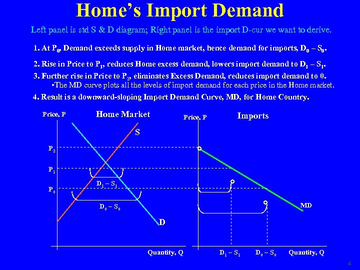
Home’s Import Demand Left panel is std S & D diagram; Right panel is the import D-cur we want to derive. 1. At P 0, Demand exceeds supply in Home market, hence demand for imports, D 0 – S 0. 2. Rise in Price to P 1, reduces Home excess demand, lowers import demand to D 1 – S 1. 3. Further rise in Price to P 2, eliminates Excess Demand, reduces import demand to 0. • The MD curve plots all the levels of import demand for each price in the Home market. 4. Result is a downward-sloping Import Demand Curve, MD, for Home Country. Price, P Home Market Price, P Imports S P 2 P 1 P 0 D 1 – S 1 MD D 0 – S 0 D Quantity, Q D 1 – S 1 D 0 – S 0 Quantity, Q 4
XS = MS curve • Do Export Supply Curve = Home’s import supply curve. – This tells us how much a nation would export for any given domestic price 5
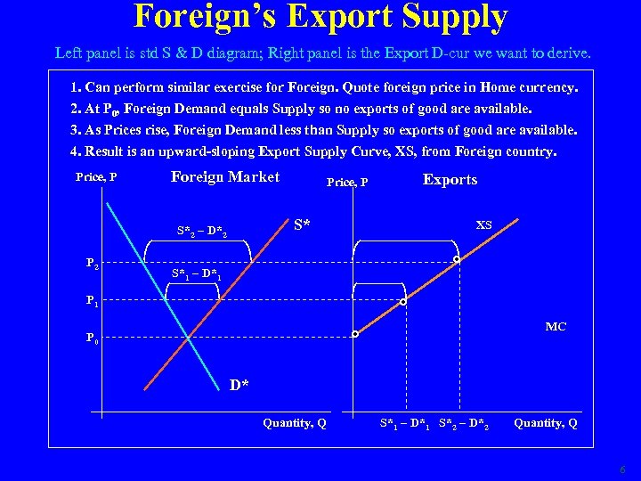
Foreign’s Export Supply Left panel is std S & D diagram; Right panel is the Export D-cur we want to derive. 1. Can perform similar exercise for Foreign. Quote foreign price in Home currency. 2. At P 0, Foreign Demand equals Supply so no exports of good are available. 3. As Prices rise, Foreign Demand less than Supply so exports of good are available. 4. Result is an upward-sloping Export Supply Curve, XS, from Foreign country. Price, P Foreign Market S* S*2 – D*2 P 2 Price, P Exports XS S*1 – D*1 P 1 MC P 0 D* Quantity, Q S*1 – D*1 S*2 – D*2 Quantity, Q 6
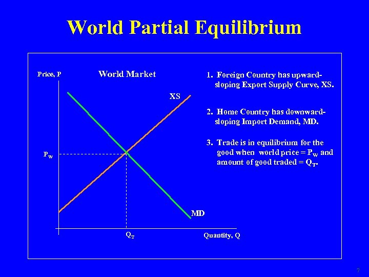
World Partial Equilibrium Price, P World Market 1. Foreign Country has upwardsloping Export Supply Curve, XS. XS 2. Home Country has downwardsloping Import Demand, MD. 3. Trade is in equilibrium for the good when world price = PW and amount of good traded = QT. PW MD QT Quantity, Q 7
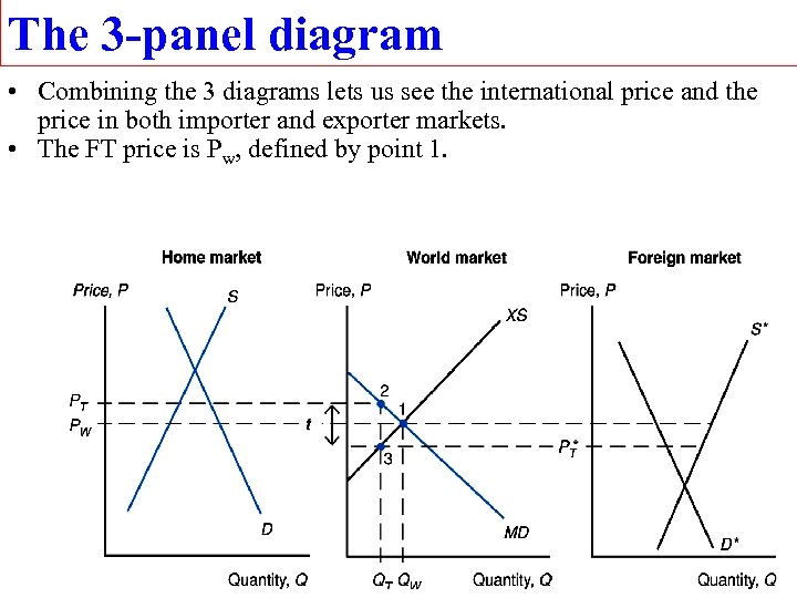
The 3 -panel diagram • Combining the 3 diagrams lets us see the international price and the price in both importer and exporter markets. • The FT price is Pw, defined by point 1. 8
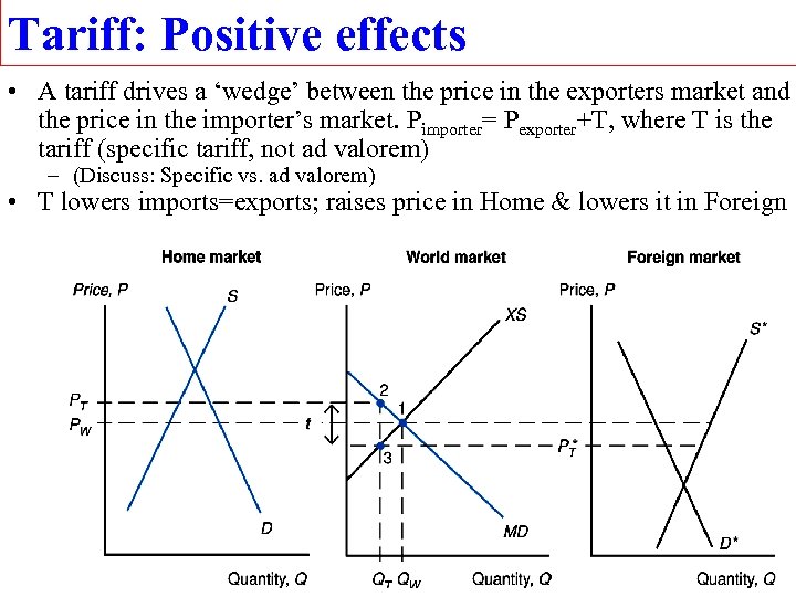
Tariff: Positive effects • A tariff drives a ‘wedge’ between the price in the exporters market and the price in the importer’s market. Pimporter= Pexporter+T, where T is the tariff (specific tariff, not ad valorem) – (Discuss: Specific vs. ad valorem) • T lowers imports=exports; raises price in Home & lowers it in Foreign 9
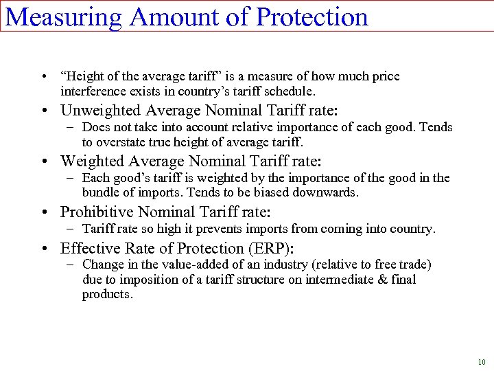
Measuring Amount of Protection • “Height of the average tariff” is a measure of how much price interference exists in country’s tariff schedule. • Unweighted Average Nominal Tariff rate: – Does not take into account relative importance of each good. Tends to overstate true height of average tariff. • Weighted Average Nominal Tariff rate: – Each good’s tariff is weighted by the importance of the good in the bundle of imports. Tends to be biased downwards. • Prohibitive Nominal Tariff rate: – Tariff rate so high it prevents imports from coming into country. • Effective Rate of Protection (ERP): – Change in the value-added of an industry (relative to free trade) due to imposition of a tariff structure on intermediate & final products. 10
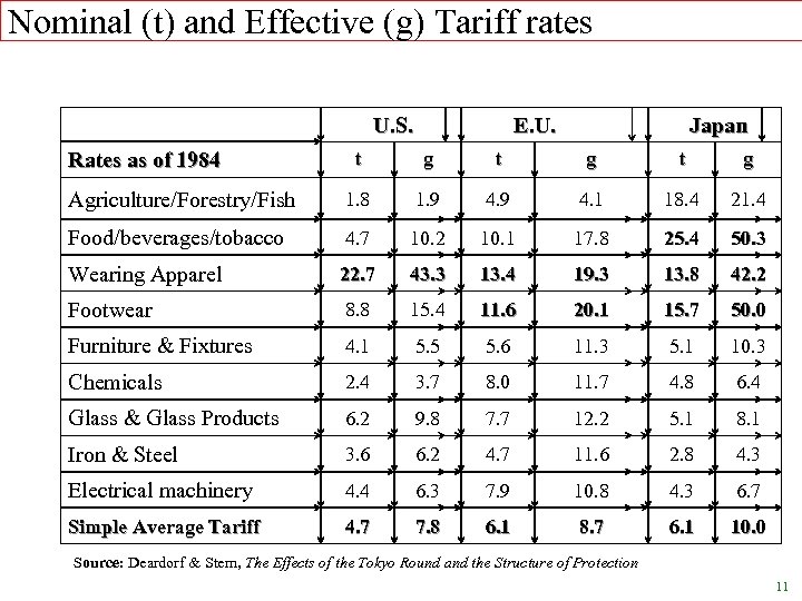
Nominal (t) and Effective (g) Tariff rates U. S. E. U. Japan t g t g Agriculture/Forestry/Fish 1. 8 1. 9 4. 1 18. 4 21. 4 Food/beverages/tobacco 4. 7 10. 2 10. 1 17. 8 25. 4 50. 3 Wearing Apparel 22. 7 43. 3 13. 4 19. 3 13. 8 42. 2 Footwear 8. 8 15. 4 11. 6 20. 1 15. 7 50. 0 Furniture & Fixtures 4. 1 5. 5 5. 6 11. 3 5. 1 10. 3 Chemicals 2. 4 3. 7 8. 0 11. 7 4. 8 6. 4 Glass & Glass Products 6. 2 9. 8 7. 7 12. 2 5. 1 8. 1 Iron & Steel 3. 6 6. 2 4. 7 11. 6 2. 8 4. 3 Electrical machinery 4. 4 6. 3 7. 9 10. 8 4. 3 6. 7 Simple Average Tariff 4. 7 7. 8 6. 1 8. 7 6. 1 10. 0 Rates as of 1984 Source: Deardorf & Stern, The Effects of the Tokyo Round and the Structure of Protection 11
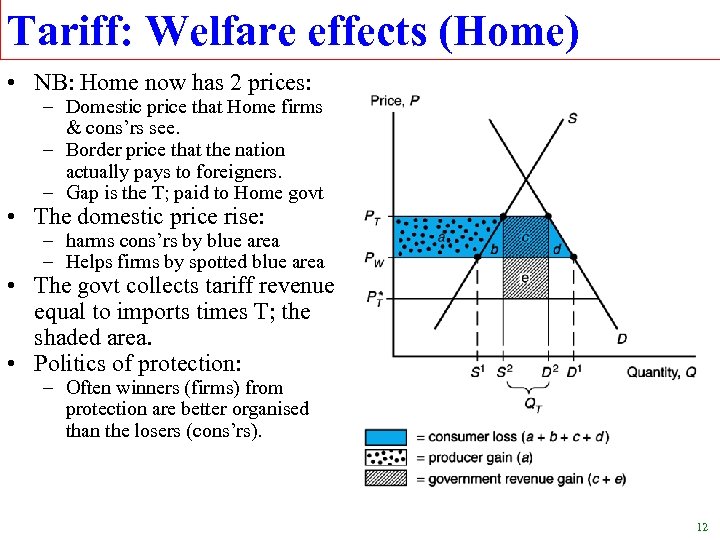
Tariff: Welfare effects (Home) • NB: Home now has 2 prices: – Domestic price that Home firms & cons’rs see. – Border price that the nation actually pays to foreigners. – Gap is the T; paid to Home govt • The domestic price rise: – harms cons’rs by blue area – Helps firms by spotted blue area • The govt collects tariff revenue equal to imports times T; the shaded area. • Politics of protection: – Often winners (firms) from protection are better organised than the losers (cons’rs). 12
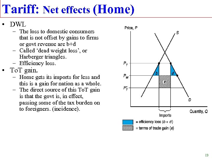
Tariff: Net effects (Home) • DWL – The loss to domestic consumers that is not offset by gains to firms or govt revenue are b+d – Called ‘dead weight loss’, or Harberger triangles. – Efficiency loss. • To. T gain. – Home gets imports for less and this is a gain for nation as a whole. – The direct source of this To. T gain is that the govt is, in effect, passing some of the tax burden on to foreigners. (incidence). 13
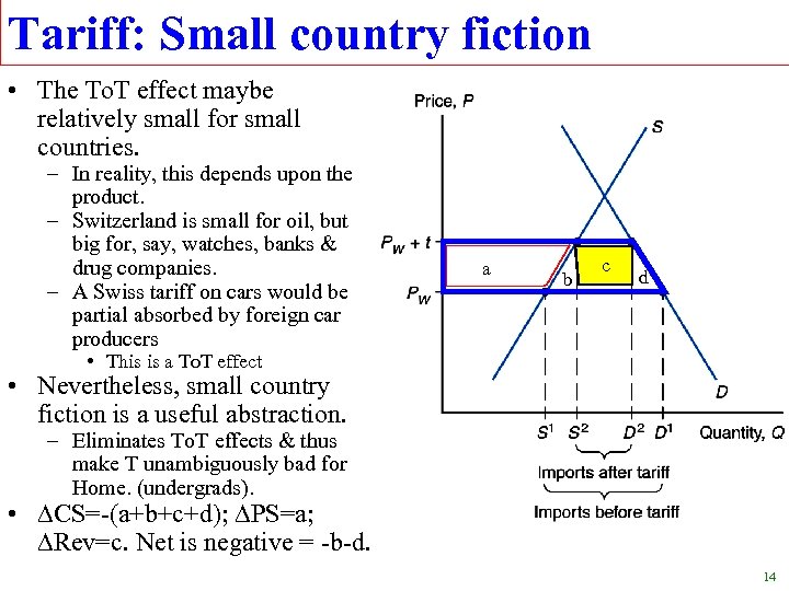
Tariff: Small country fiction • The To. T effect maybe relatively small for small countries. – In reality, this depends upon the product. – Switzerland is small for oil, but big for, say, watches, banks & drug companies. – A Swiss tariff on cars would be partial absorbed by foreign car producers a b c d • This is a To. T effect • Nevertheless, small country fiction is a useful abstraction. – Eliminates To. T effects & thus make T unambiguously bad for Home. (undergrads). • CS=-(a+b+c+d); PS=a; Rev=c. Net is negative = -b-d. 14
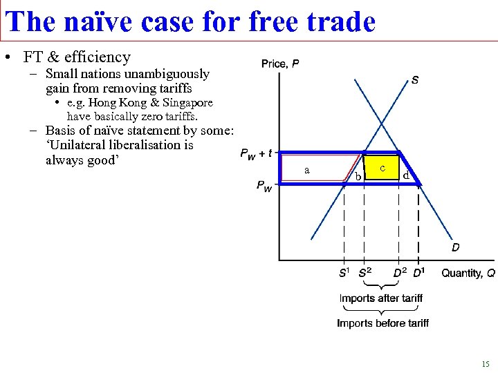
The naïve case for free trade • FT & efficiency – Small nations unambiguously gain from removing tariffs • e. g. Hong Kong & Singapore have basically zero tariffs. – Basis of naïve statement by some: ‘Unilateral liberalisation is always good’ a b c d 15
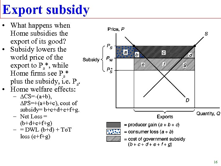
Export subsidy • What happens when Home subsidies the export of its good? • Subsidy lowers the world price of the export to Ps*, while Home firms see Ps* plus the subsidy, i. e. Ps. • Home welfare effects: – CS=-(a+b), PS=+(a+b+c), cost of subsidy= b+c+d+e+f+g. – Net Loss = (b+d+e+f+g) – = DWL (b+d) + To. T loss (e+f+g) 16
Export tax like import tariff, G. E. • This is called ‘Lerner’s symmetry’ • The basic point is almost trivial. • With two goods and only relative prices mattering, the impact on the relative price of raising the numerator is the same as lowering the denominator. • Import tariff raises the internal price of imports relative to exports. • Export tax lowers the internal price of exports to imports (since now domestic export firm sell less abroad and more at home, so home price falls). • In the diagram … 17
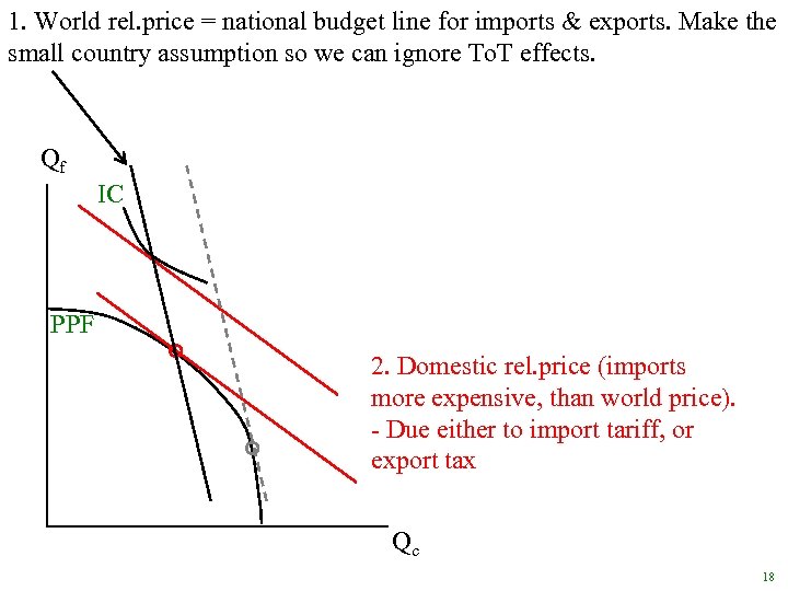
1. World rel. price = national budget line for imports & exports. Make the small country assumption so we can ignore To. T effects. Qf IC PPF 2. Domestic rel. price (imports more expensive, than world price). - Due either to import tariff, or export tax Qc 18
Non-tariff Barriers (NTBs) • Bit of history on terminology. • Most common form of a Non-Tariff Barrier is a QR=quantitative restriction. – an import quota is one common QR, it restricts the quantity of good imported. – Requiring an import license is a common means of implementing. • Import Quota – Restricts quantity of good imported during a year. – Effect is to increase home price of the good over free trade. – Market effects identical to a specific tariff (if perfect competition). • In fact, any quota can be mimicked by an equivalent tariff, so we often speak of the ‘tariffequivalent’ of the QR. – Welfare effects differ because gov’t does not necessarily receive revenue as under a tariff. • ‘Quota rents’= buy low, sell high. • Depends who has the rights to the import licenses – Govt may gain revenue if auctions off import licenses, – otherwise additional revenue received by domestic imports, or foreign exporters. • Other types of QRs (many illegal now under the WTO; called ‘grey area’ measures under the GATT) – Voluntary Export Restraint (VER’s) • Foreign supplier “voluntarily” agrees to restrict quantity imported. • Usually a political agreement so Home does not look protectionist. • Market effects identical to an import quota, but welfare effects differ as foreign firms receive additional profit, Home gov’t receives nothing. – VRAs, OMA • Application: How economic sanctions can make the target regime rich. 19
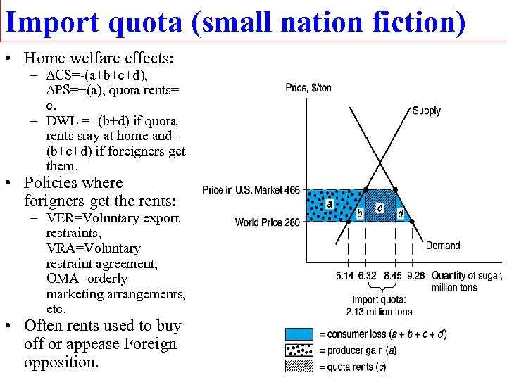
Import quota (small nation fiction) • Home welfare effects: – CS=-(a+b+c+d), PS=+(a), quota rents= c. – DWL = -(b+d) if quota rents stay at home and (b+c+d) if foreigners get them. • Policies where forigners get the rents: – VER=Voluntary export restraints, VRA=Voluntary restraint agreement, OMA=orderly marketing arrangements, etc. • Often rents used to buy off or appease Foreign opposition. 20
NTBs & corruption • Any time imports are constrained, a buy-low-sellhigh opportunity arises. • With a tariff, govt exploits this • With NTBs, who knows? – Invitation to corruption of domestic govt officials who allocate the import licenses or other control devices, foreign export firms, domestic smugglers, etc. • Lack of transparency – How much protection is provided? • Domestic industry prefers due to certainty of import level. 21
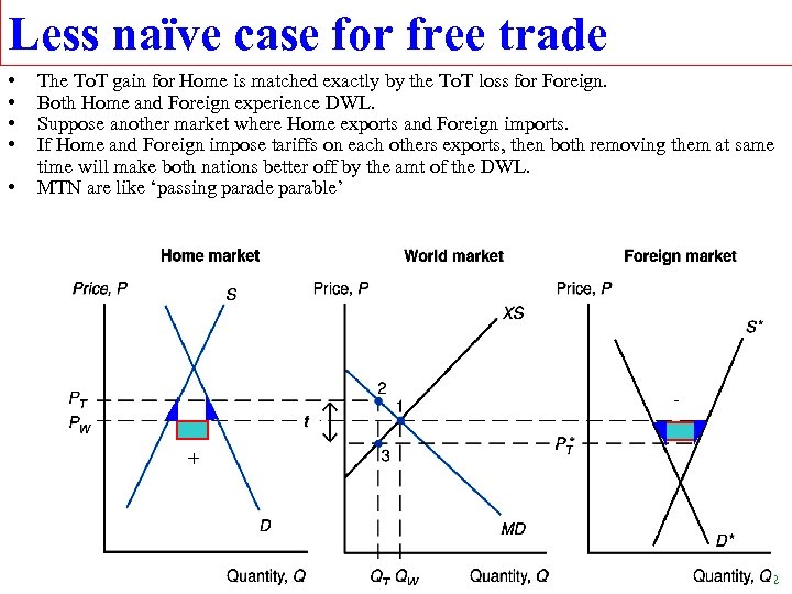
Less naïve case for free trade • • • The To. T gain for Home is matched exactly by the To. T loss for Foreign. Both Home and Foreign experience DWL. Suppose another market where Home exports and Foreign imports. If Home and Foreign impose tariffs on each others exports, then both removing them at same time will make both nations better off by the amt of the DWL. MTN are like ‘passing parade parable’ + 22
‘dynamic’ GFT • These efficiency gains are multiplied by other gains such as increased economies of scale, and proinvestment effects. • Working these out can be complex, but basic idea is simple. • Improved ‘static’ efficiency improves a nation’s investment climate, so more investment gets done. • The initial static GFT is multiplied by trade-induced investment-led growth. 23
Political argument • Protection is a way of allocating resources in the economy, i. e. influencing production and dist’n of welfare. • Markets are imperfect so there may be an economic argument for protection, but politicians are also imperfect, so the question is: – Which is more imperfect? Politically chosen import prices, or market chosen? • Powerful special interest groups often manage to get govts to put in policies that help few rich and harm many less rich consumers. – They often use populist arguments and play of ignorance of voters. 24
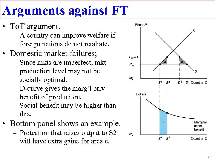
Arguments against FT • To. T argument. – A country can improve welfare if foreign nations do not retaliate. • Domestic market failures; – Since mkts are imperfect, mkt production level may not be socially optimal. – D-curve gives the marg’l priv benefit of produciton. – Social benefit may be higher than this. • Bottom panel shows an example. – Protection that raises output to S 2 will have extra gains for area c. 25
End 26
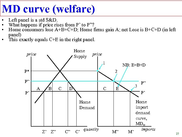
MD curve (welfare) • Left panel is a std S&D. • What happens if price rises from P’ to P”? • Home consumers lose A+B+C+D; Home firms gain A; net Lose is B+C+D (in left panel) • This exactly equals C+E in the right panel. Home Supply price 1 P* NB: E=B+D 2 P” P’ A B C D C 3 E P’ Home Demand Z’ Z” C” C’ quantity M” P” M’ Home import demand curve, MDH imports 27
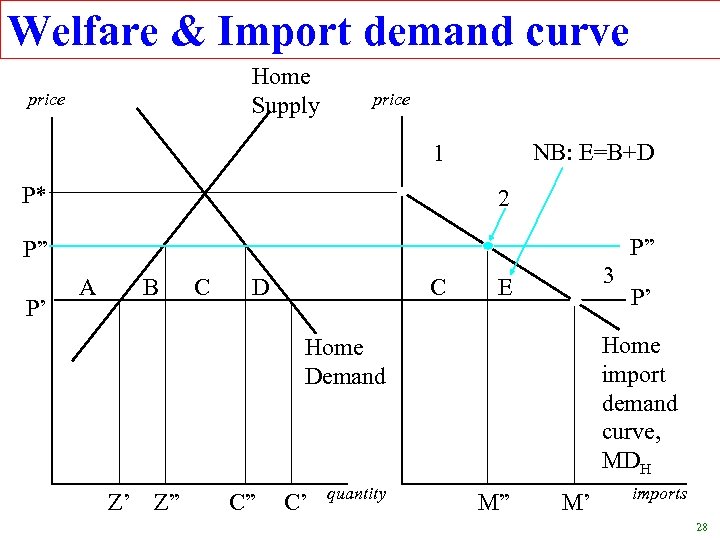
Welfare & Import demand curve Home Supply price NB: E=B+D 1 P* 2 P” P” P’ A B C D C 3 E Home import demand curve, MDH Home Demand Z’ Z” C” C’ quantity P’ M” M’ imports 28
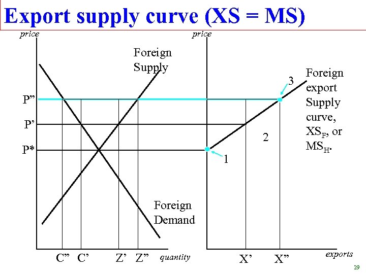
Export supply curve (XS = MS) price Foreign Supply P” P’ 2 P* 1 Foreign 3 export Supply curve, XSF, or MSH. Foreign Demand C” C’ Z’ Z” quantity X’ X” exports 29
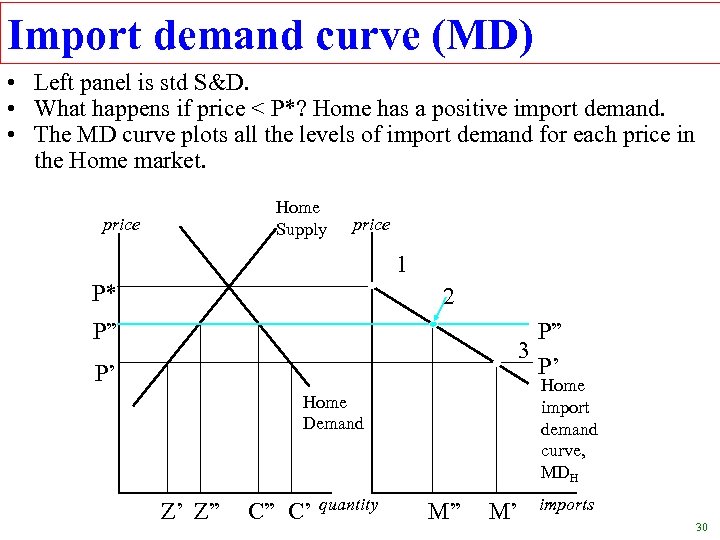
Import demand curve (MD) • Left panel is std S&D. • What happens if price < P*? Home has a positive import demand. • The MD curve plots all the levels of import demand for each price in the Home market. Home Supply price 1 P* 2 P” 3 P’ P” P’ Home import demand curve, MDH Home Demand Z’ Z” C” C’ quantity M” M’ imports 30
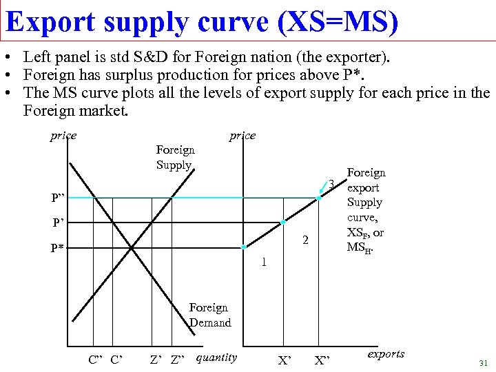
Export supply curve (XS=MS) • Left panel is std S&D for Foreign nation (the exporter). • Foreign has surplus production for prices above P*. • The MS curve plots all the levels of export supply for each price in the Foreign market. price Foreign Supply P” P’ 2 P* 1 Foreign 3 export Supply curve, XSF, or MSH. Foreign Demand C” C’ Z’ Z” quantity X’ X” exports 31
8791b85c7b994569fbca5cfef620de26.ppt