a56bc04cb42997f8dfbedcf82f64d1c9.ppt
- Количество слайдов: 80
Business Statistics: A Decision-Making Approach 8 th Edition Chapter 15 Multiple Regression Analysis and Model Building Copyright © 2011 Pearson Education, Inc. publishing as Prentice Hall 15 -1
Chapter Goals After completing this chapter, you should be able to: n n Explain model building using multiple regression analysis Apply multiple regression analysis to business decision-making situations Analyze and interpret the computer output for a multiple regression model Test the significance of the independent variables in a multiple regression model Copyright © 2011 Pearson Education, Inc. publishing as Prentice Hall 2
Chapter Goals (continued) After completing this chapter, you should be able to: n Recognize potential problems in multiple regression analysis and take steps to correct the problems n Incorporate qualitative variables into the regression model by using dummy variables n Use variable transformations to model nonlinear relationships n Test if the coefficients of a regression model are useful Copyright © 2011 Pearson Education, Inc. publishing as Prentice Hall 3
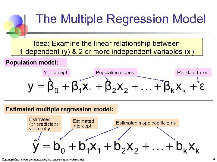
The Multiple Regression Model Idea: Examine the linear relationship between 1 dependent (y) & 2 or more independent variables (xi) Population model: Y-intercept Population slopes Random Error Estimated multiple regression model: Estimated (or predicted) value of y Estimated intercept Copyright © 2011 Pearson Education, Inc. publishing as Prentice Hall Estimated slope coefficients 4
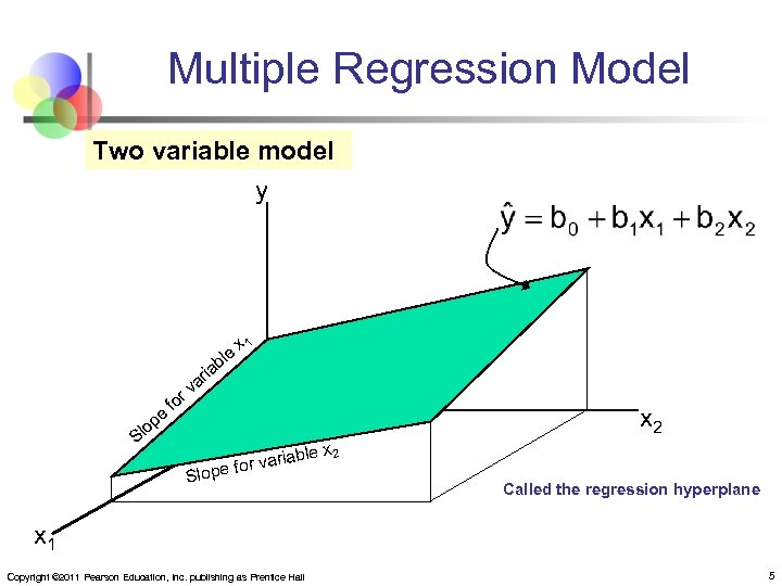
Multiple Regression Model Two variable model y ia e p lo r fo r va e bl x 1 S x 2 le x 2 ariab e for v Slop Called the regression hyperplane x 1 Copyright © 2011 Pearson Education, Inc. publishing as Prentice Hall 5
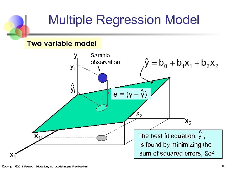
Multiple Regression Model Two variable model y yi Sample observation < < yi e = (y – y) x 2 i x 1 Copyright © 2011 Pearson Education, Inc. publishing as Prentice Hall < x 1 i x 2 The best fit equation, y , is found by minimizing the sum of squared errors, e 2 6
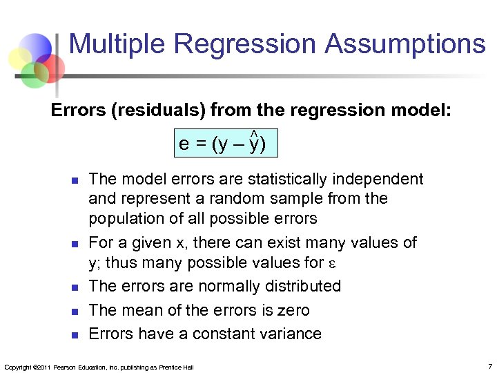
Multiple Regression Assumptions Errors (residuals) from the regression model: < e = (y – y) n n n The model errors are statistically independent and represent a random sample from the population of all possible errors For a given x, there can exist many values of y; thus many possible values for The errors are normally distributed The mean of the errors is zero Errors have a constant variance Copyright © 2011 Pearson Education, Inc. publishing as Prentice Hall 7
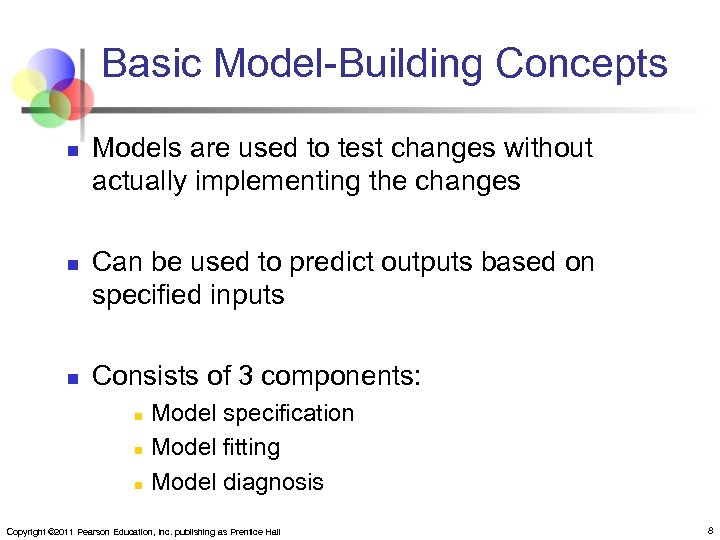
Basic Model-Building Concepts n n n Models are used to test changes without actually implementing the changes Can be used to predict outputs based on specified inputs Consists of 3 components: n n n Model specification Model fitting Model diagnosis Copyright © 2011 Pearson Education, Inc. publishing as Prentice Hall 8
Model Specification n n Sometimes referred to as model identification Is a process for establishing the framework for the model n n n Decide what you want to do and select the dependent variable (y) Determine the potential independent variables (x) for your model Gather sample data (observations) for all variables Copyright © 2011 Pearson Education, Inc. publishing as Prentice Hall 9
Model Building n n n Process of actually constructing the equation for the data May include some or all of the independent variables (x) The goal is to explain the variation in the dependent variable (y) with the selected independent variables (x) Copyright © 2011 Pearson Education, Inc. publishing as Prentice Hall 10
Model Diagnosis n n Analyzing the quality of the model (perform diagnostic checks) Assess the extent to which the assumptions appear to be satisfied If unacceptable, begin the model-building process again Should use the simplest model available to meet needs n The goal is to help you make better decisions Copyright © 2011 Pearson Education, Inc. publishing as Prentice Hall 11
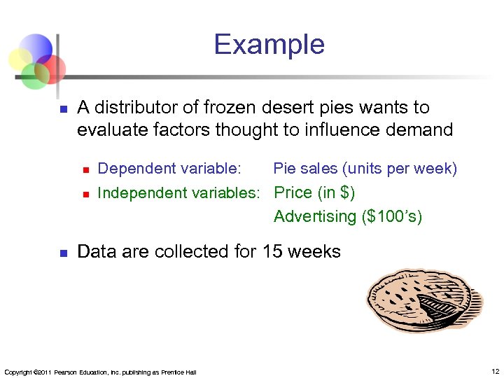
Example n A distributor of frozen desert pies wants to evaluate factors thought to influence demand n n Dependent variable: Pie sales (units per week) Independent variables: Price (in $) Advertising ($100’s) n Data are collected for 15 weeks Copyright © 2011 Pearson Education, Inc. publishing as Prentice Hall 12
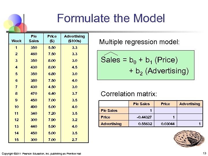
Formulate the Model Week Pie Sales Price ($) Advertising ($100 s) 1 350 5. 50 3. 3 2 460 7. 50 3. 3 3 350 8. 00 3. 0 4 430 8. 00 4. 5 5 350 6. 80 3. 0 6 380 7. 50 4. 0 7 430 4. 50 3. 0 8 470 6. 40 3. 7 9 450 7. 00 3. 5 10 490 5. 00 4. 0 11 340 7. 20 3. 5 12 300 7. 90 3. 2 13 440 5. 90 4. 0 14 450 5. 00 3. 5 15 300 7. 00 2. 7 Copyright © 2011 Pearson Education, Inc. publishing as Prentice Hall Multiple regression model: Sales = b 0 + b 1 (Price) + b 2 (Advertising) Correlation matrix: Pie Sales Price Advertising 1 -0. 44327 1 0. 55632 0. 03044 1 13
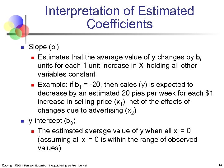
Interpretation of Estimated Coefficients n n Slope (bi) n Estimates that the average value of y changes by b i units for each 1 unit increase in Xi holding all other variables constant n Example: if b 1 = -20, then sales (y) is expected to decrease by an estimated 20 pies per week for each $1 increase in selling price (x 1), net of the effects of changes due to advertising (x 2) y-intercept (b 0) n The estimated average value of y when all xi = 0 (assuming all xi = 0 is within the range of observed values) Copyright © 2011 Pearson Education, Inc. publishing as Prentice Hall 14
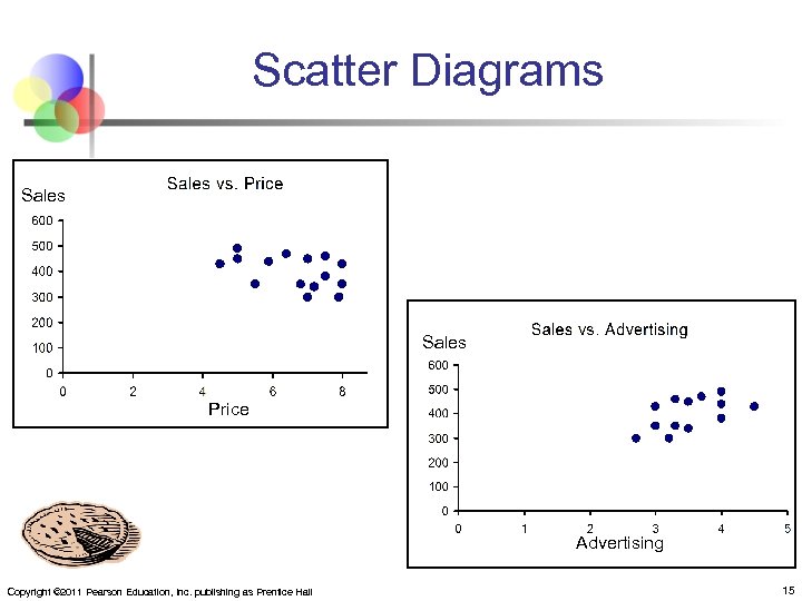
Scatter Diagrams Sales Price Advertising Copyright © 2011 Pearson Education, Inc. publishing as Prentice Hall 15
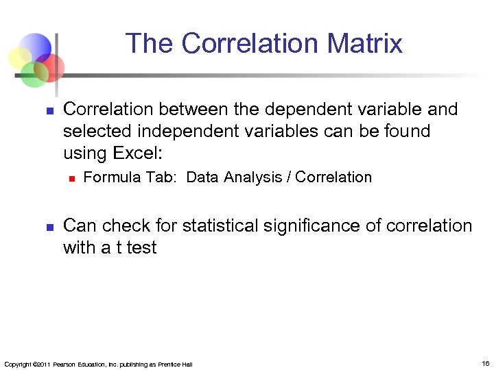
The Correlation Matrix n Correlation between the dependent variable and selected independent variables can be found using Excel: n n Formula Tab: Data Analysis / Correlation Can check for statistical significance of correlation with a t test Copyright © 2011 Pearson Education, Inc. publishing as Prentice Hall 16
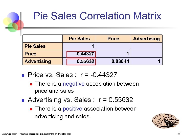
Pie Sales Correlation Matrix Pie Sales Price Advertising n Advertising 1 -0. 44327 1 0. 55632 0. 03044 1 Price vs. Sales : r = -0. 44327 n n Price There is a negative association between price and sales Advertising vs. Sales : r = 0. 55632 n There is a positive association between advertising and sales Copyright © 2011 Pearson Education, Inc. publishing as Prentice Hall 17
Estimating a Multiple Linear Regression Equation n n Computer software is generally used to generate the coefficients and measures of goodness of fit for multiple regression Excel: n n Data / Data Analysis / Regression PHStat: n Add-Ins / PHStat / Regression / Multiple Regression… Copyright © 2011 Pearson Education, Inc. publishing as Prentice Hall 18
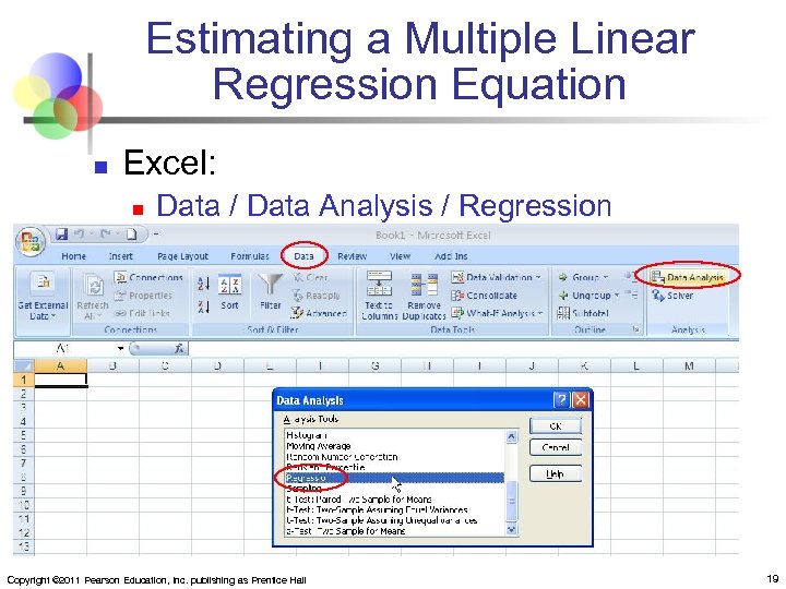
Estimating a Multiple Linear Regression Equation n Excel: n Data / Data Analysis / Regression Copyright © 2011 Pearson Education, Inc. publishing as Prentice Hall 19
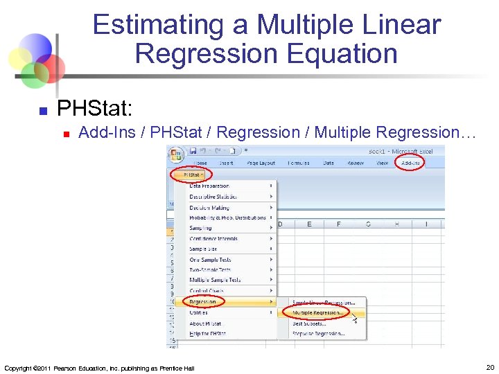
Estimating a Multiple Linear Regression Equation n PHStat: n Add-Ins / PHStat / Regression / Multiple Regression… Copyright © 2011 Pearson Education, Inc. publishing as Prentice Hall 20
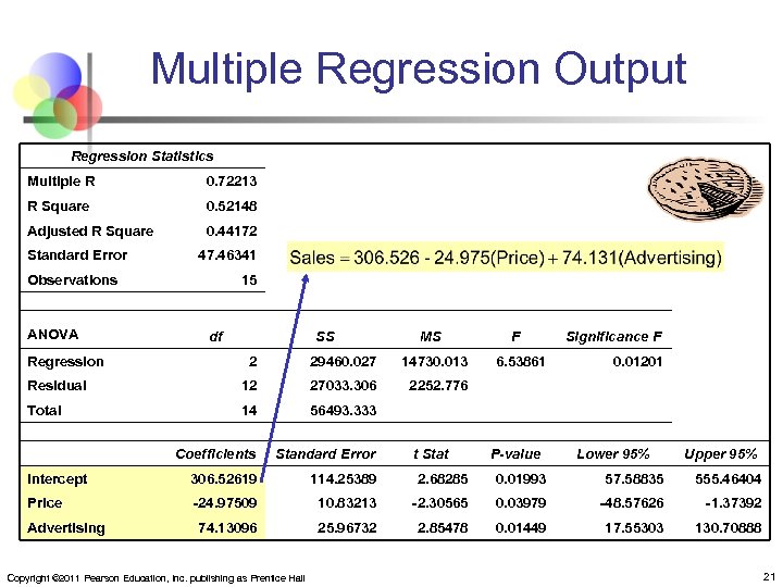
Multiple Regression Output Regression Statistics Multiple R 0. 72213 R Square 0. 52148 Adjusted R Square 0. 44172 Standard Error 47. 46341 Observations ANOVA 15 df Regression SS MS F Significance F 2 29460. 027 14730. 013 Residual 12 27033. 306 2252. 776 Total 14 56493. 333 Coefficients Standard Error Intercept 306. 52619 114. 25389 2. 68285 0. 01993 57. 58835 555. 46404 Price -24. 97509 10. 83213 -2. 30565 0. 03979 -48. 57626 -1. 37392 74. 13096 25. 96732 2. 85478 0. 01449 17. 55303 130. 70888 Advertising Copyright © 2011 Pearson Education, Inc. publishing as Prentice Hall 6. 53861 t Stat 0. 01201 P-value Lower 95% Upper 95% 21
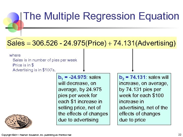
The Multiple Regression Equation where Sales is in number of pies per week Price is in $ Advertising is in $100’s. b 1 = -24. 975: sales will decrease, on average, by 24. 975 pies per week for each $1 increase in selling price, net of the effects of changes due to advertising Copyright © 2011 Pearson Education, Inc. publishing as Prentice Hall b 2 = 74. 131: sales will increase, on average, by 74. 131 pies per week for each $100 increase in advertising, net of the effects of changes due to price 22
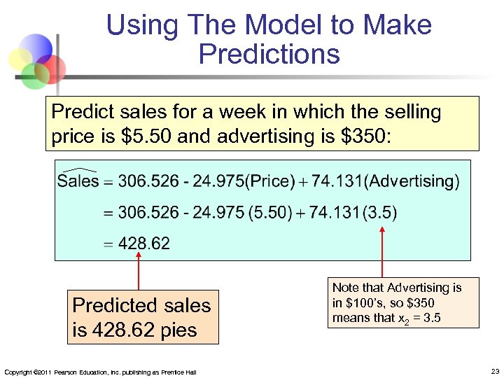
Using The Model to Make Predictions Predict sales for a week in which the selling price is $5. 50 and advertising is $350: Predicted sales is 428. 62 pies Copyright © 2011 Pearson Education, Inc. publishing as Prentice Hall Note that Advertising is in $100’s, so $350 means that x 2 = 3. 5 23
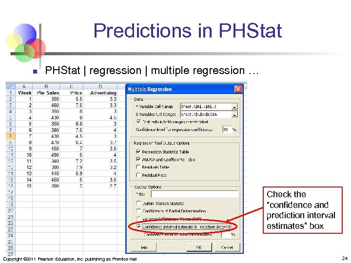
Predictions in PHStat | regression | multiple regression … Check the “confidence and prediction interval estimates” box Copyright © 2011 Pearson Education, Inc. publishing as Prentice Hall 24
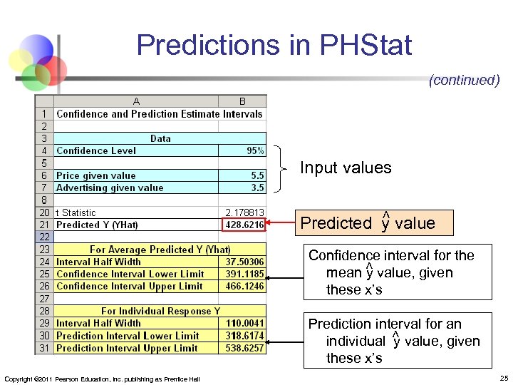
Predictions in PHStat (continued) Input values < Predicted y value < Confidence interval for the mean y value, given these x’s < Prediction interval for an individual y value, given these x’s Copyright © 2011 Pearson Education, Inc. publishing as Prentice Hall 25
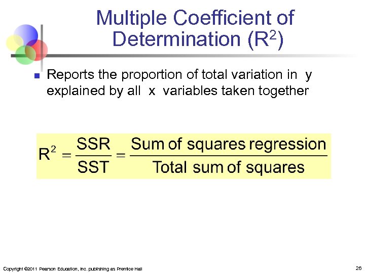
Multiple Coefficient of Determination (R 2) n Reports the proportion of total variation in y explained by all x variables taken together Copyright © 2011 Pearson Education, Inc. publishing as Prentice Hall 26
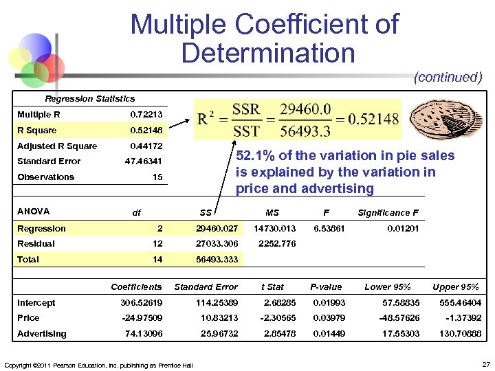
Multiple Coefficient of Determination (continued) Regression Statistics Multiple R 0. 72213 R Square 0. 52148 Adjusted R Square 0. 44172 Standard Error Observations ANOVA 52. 1% of the variation in pie sales is explained by the variation in price and advertising 47. 46341 15 df Regression SS MS F Significance F 2 29460. 027 14730. 013 Residual 12 27033. 306 2252. 776 Total 14 56493. 333 Coefficients Standard Error Intercept 306. 52619 114. 25389 2. 68285 0. 01993 57. 58835 555. 46404 Price -24. 97509 10. 83213 -2. 30565 0. 03979 -48. 57626 -1. 37392 74. 13096 25. 96732 2. 85478 0. 01449 17. 55303 130. 70888 Advertising Copyright © 2011 Pearson Education, Inc. publishing as Prentice Hall 6. 53861 t Stat 0. 01201 P-value Lower 95% Upper 95% 27
Adjusted R 2 n n R 2 never decreases when a new x variable is added to the model n This can be a disadvantage when comparing models What is the net effect of adding a new variable? n We lose a degree of freedom when a new x variable is added n Did the new x variable add enough explanatory power to offset the loss of one degree of freedom? Copyright © 2011 Pearson Education, Inc. publishing as Prentice Hall 28
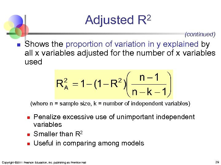
Adjusted R 2 (continued) n Shows the proportion of variation in y explained by all x variables adjusted for the number of x variables used (where n = sample size, k = number of independent variables) n n n Penalize excessive use of unimportant independent variables Smaller than R 2 Useful in comparing among models Copyright © 2011 Pearson Education, Inc. publishing as Prentice Hall 29
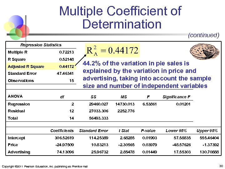
Multiple Coefficient of Determination (continued) Regression Statistics Multiple R 0. 72213 R Square 0. 52148 Adjusted R Square 0. 44172 Standard Error 47. 46341 Observations ANOVA 15 44. 2% of the variation in pie sales is explained by the variation in price and advertising, taking into account the sample size and number of independent variables df Regression SS MS F Significance F 2 29460. 027 14730. 013 Residual 12 27033. 306 2252. 776 Total 14 56493. 333 Coefficients Standard Error Intercept 306. 52619 114. 25389 2. 68285 0. 01993 57. 58835 555. 46404 Price -24. 97509 10. 83213 -2. 30565 0. 03979 -48. 57626 -1. 37392 74. 13096 25. 96732 2. 85478 0. 01449 17. 55303 130. 70888 Advertising Copyright © 2011 Pearson Education, Inc. publishing as Prentice Hall 6. 53861 t Stat 0. 01201 P-value Lower 95% Upper 95% 30
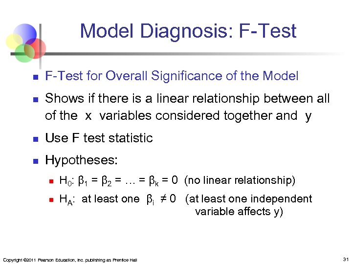
Model Diagnosis: F-Test n n F-Test for Overall Significance of the Model Shows if there is a linear relationship between all of the x variables considered together and y n Use F test statistic n Hypotheses: n n H 0: β 1 = β 2 = … = βk = 0 (no linear relationship) HA: at least one βi ≠ 0 (at least one independent variable affects y) Copyright © 2011 Pearson Education, Inc. publishing as Prentice Hall 31
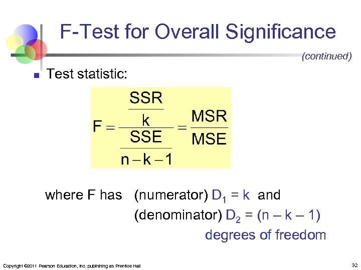
F-Test for Overall Significance (continued) n Test statistic: where F has (numerator) D 1 = k and (denominator) D 2 = (n – k – 1) degrees of freedom Copyright © 2011 Pearson Education, Inc. publishing as Prentice Hall 32
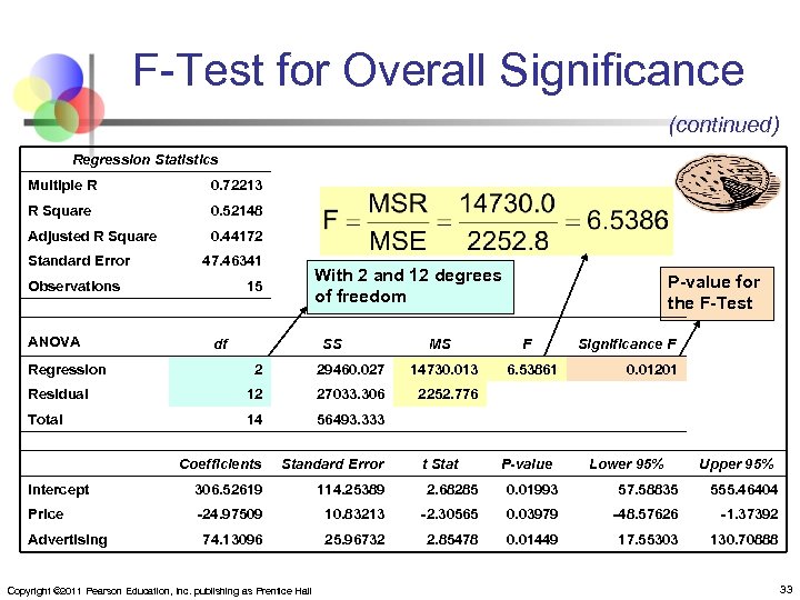
F-Test for Overall Significance (continued) Regression Statistics Multiple R 0. 72213 R Square 0. 52148 Adjusted R Square 0. 44172 Standard Error 47. 46341 Observations ANOVA With 2 and 12 degrees of freedom 15 df Regression SS MS P-value for the F-Test F Significance F 2 29460. 027 14730. 013 Residual 12 27033. 306 2252. 776 Total 14 56493. 333 Coefficients Standard Error Intercept 306. 52619 114. 25389 2. 68285 0. 01993 57. 58835 555. 46404 Price -24. 97509 10. 83213 -2. 30565 0. 03979 -48. 57626 -1. 37392 74. 13096 25. 96732 2. 85478 0. 01449 17. 55303 130. 70888 Advertising Copyright © 2011 Pearson Education, Inc. publishing as Prentice Hall 6. 53861 t Stat 0. 01201 P-value Lower 95% Upper 95% 33
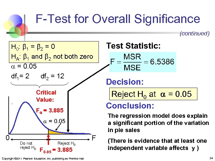
F-Test for Overall Significance (continued) H 0: β 1 = β 2 = 0 HA: β 1 and β 2 not both zero = 0. 05 df 1= 2 df 2 = 12 Critical Value: F = 3. 885 Do not reject H 0 Reject H 0 F 0. 05 = 3. 885 Copyright © 2011 Pearson Education, Inc. publishing as Prentice Hall Decision: Reject H 0 at = 0. 05 Conclusion: The regression model does explain a significant portion of the variation in pie sales = 0. 05 0 Test Statistic: F (There is evidence that at least one independent variable affects y ) 34
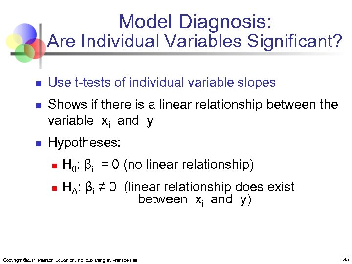
Model Diagnosis: Are Individual Variables Significant? n n n Use t-tests of individual variable slopes Shows if there is a linear relationship between the variable xi and y Hypotheses: n n H 0: βi = 0 (no linear relationship) HA: βi ≠ 0 (linear relationship does exist between xi and y) Copyright © 2011 Pearson Education, Inc. publishing as Prentice Hall 35
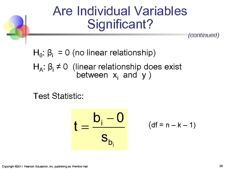
Are Individual Variables Significant? (continued) H 0: βi = 0 (no linear relationship) HA: βi ≠ 0 (linear relationship does exist between xi and y ) Test Statistic: (df = n – k – 1) Copyright © 2011 Pearson Education, Inc. publishing as Prentice Hall 36
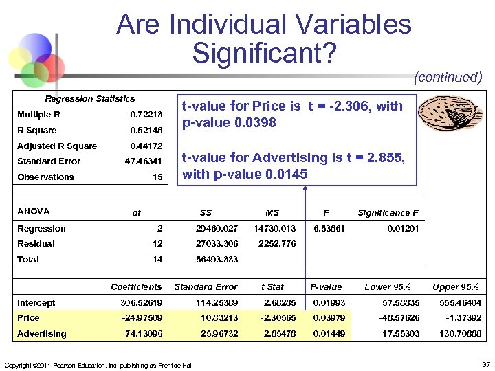
Are Individual Variables Significant? (continued) Regression Statistics Multiple R 0. 72213 R Square 0. 52148 Adjusted R Square 0. 44172 Standard Error 47. 46341 Observations ANOVA 15 t-value for Price is t = -2. 306, with p-value 0. 0398 t-value for Advertising is t = 2. 855, with p-value 0. 0145 df Regression SS MS F Significance F 2 29460. 027 14730. 013 Residual 12 27033. 306 2252. 776 Total 14 56493. 333 Coefficients Standard Error Intercept 306. 52619 114. 25389 2. 68285 0. 01993 57. 58835 555. 46404 Price -24. 97509 10. 83213 -2. 30565 0. 03979 -48. 57626 -1. 37392 74. 13096 25. 96732 2. 85478 0. 01449 17. 55303 130. 70888 Advertising Copyright © 2011 Pearson Education, Inc. publishing as Prentice Hall 6. 53861 t Stat 0. 01201 P-value Lower 95% Upper 95% 37
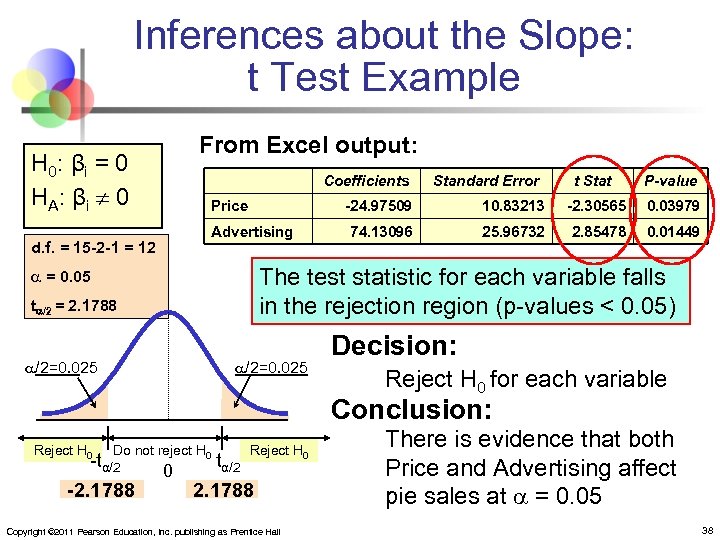
Inferences about the Slope: t Test Example From Excel output: H 0: β i = 0 HA : βi 0 Price Standard Error t Stat P-value -24. 97509 Advertising d. f. = 15 -2 -1 = 12 Coefficients 10. 83213 -2. 30565 0. 03979 74. 13096 25. 96732 2. 85478 0. 01449 The test statistic for each variable falls in the rejection region (p-values < 0. 05) = 0. 05 t /2 = 2. 1788 /2=0. 025 Decision: Reject H 0 for each variable Conclusion: Reject H 0 Do not reject H 0 -tα/2 -2. 1788 0 Reject H 0 tα/2 2. 1788 Copyright © 2011 Pearson Education, Inc. publishing as Prentice Hall There is evidence that both Price and Advertising affect pie sales at = 0. 05 38
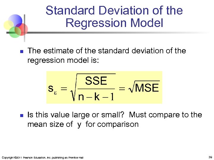
Standard Deviation of the Regression Model n n The estimate of the standard deviation of the regression model is: Is this value large or small? Must compare to the mean size of y for comparison Copyright © 2011 Pearson Education, Inc. publishing as Prentice Hall 39
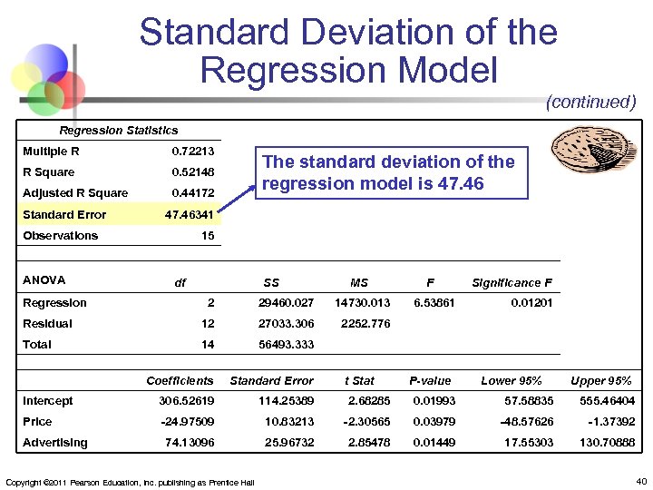
Standard Deviation of the Regression Model (continued) Regression Statistics Multiple R 0. 72213 R Square 0. 52148 Adjusted R Square 0. 44172 Standard Error 47. 46341 Observations ANOVA The standard deviation of the regression model is 47. 46 15 df Regression SS MS F Significance F 2 29460. 027 14730. 013 Residual 12 27033. 306 2252. 776 Total 14 56493. 333 Coefficients Standard Error Intercept 306. 52619 114. 25389 2. 68285 0. 01993 57. 58835 555. 46404 Price -24. 97509 10. 83213 -2. 30565 0. 03979 -48. 57626 -1. 37392 74. 13096 25. 96732 2. 85478 0. 01449 17. 55303 130. 70888 Advertising Copyright © 2011 Pearson Education, Inc. publishing as Prentice Hall 6. 53861 t Stat 0. 01201 P-value Lower 95% Upper 95% 40
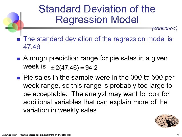
Standard Deviation of the Regression Model (continued) n n n The standard deviation of the regression model is 47. 46 A rough prediction range for pie sales in a given week is Pie sales in the sample were in the 300 to 500 per week range, so this range is probably too large to be acceptable. The analyst may want to look for additional variables that can explain more of the variation in weekly sales Copyright © 2011 Pearson Education, Inc. publishing as Prentice Hall 41
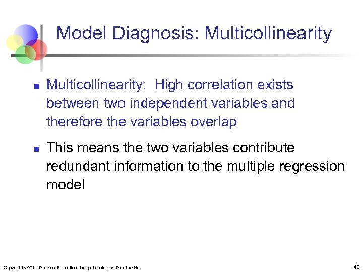
Model Diagnosis: Multicollinearity n n Multicollinearity: High correlation exists between two independent variables and therefore the variables overlap This means the two variables contribute redundant information to the multiple regression model Copyright © 2011 Pearson Education, Inc. publishing as Prentice Hall 42
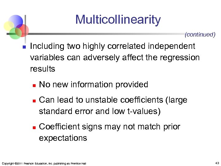
Multicollinearity (continued) n Including two highly correlated independent variables can adversely affect the regression results n n n No new information provided Can lead to unstable coefficients (large standard error and low t-values) Coefficient signs may not match prior expectations Copyright © 2011 Pearson Education, Inc. publishing as Prentice Hall 43
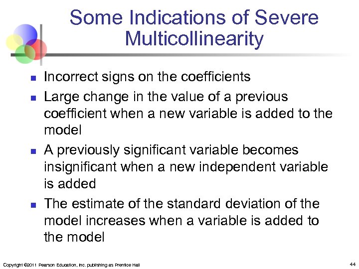
Some Indications of Severe Multicollinearity n n Incorrect signs on the coefficients Large change in the value of a previous coefficient when a new variable is added to the model A previously significant variable becomes insignificant when a new independent variable is added The estimate of the standard deviation of the model increases when a variable is added to the model Copyright © 2011 Pearson Education, Inc. publishing as Prentice Hall 44
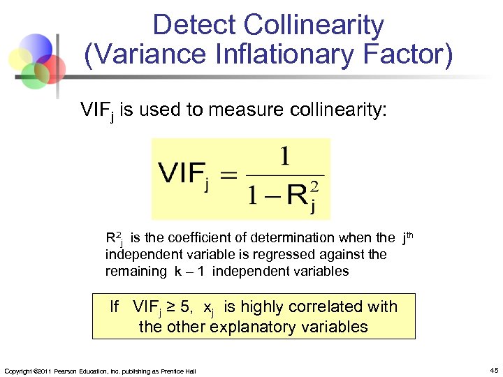
Detect Collinearity (Variance Inflationary Factor) VIFj is used to measure collinearity: R 2 j is the coefficient of determination when the jth independent variable is regressed against the remaining k – 1 independent variables If VIFj ≥ 5, xj is highly correlated with the other explanatory variables Copyright © 2011 Pearson Education, Inc. publishing as Prentice Hall 45
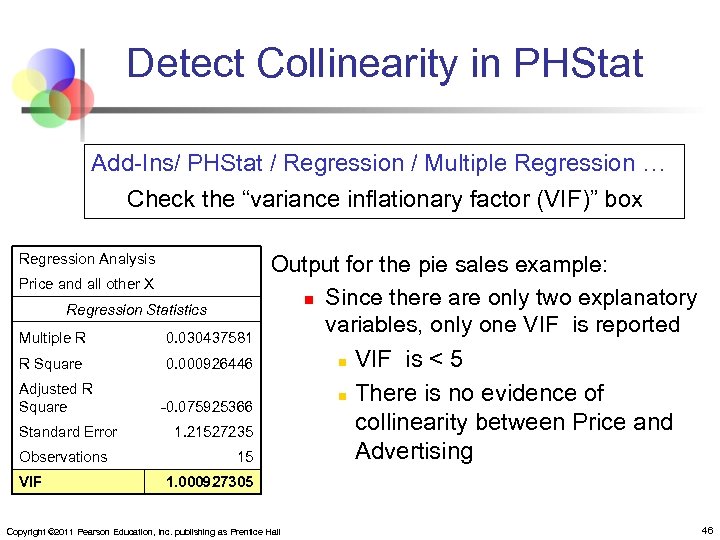
Detect Collinearity in PHStat Add-Ins/ PHStat / Regression / Multiple Regression … Check the “variance inflationary factor (VIF)” box Regression Analysis Price and all other X Regression Statistics Multiple R 0. 030437581 R Square 0. 000926446 Adjusted R Square Standard Error Observations VIF Output for the pie sales example: n Since there are only two explanatory variables, only one VIF is reported n VIF is < 5 -0. 075925366 1. 21527235 15 n There is no evidence of collinearity between Price and Advertising 1. 000927305 Copyright © 2011 Pearson Education, Inc. publishing as Prentice Hall 46
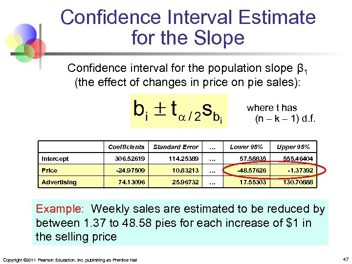
Confidence Interval Estimate for the Slope Confidence interval for the population slope β 1 (the effect of changes in price on pie sales): where t has (n – k – 1) d. f. Coefficients Standard Error … Intercept 306. 52619 114. 25389 … 57. 58835 555. 46404 Price -24. 97509 10. 83213 … -48. 57626 -1. 37392 74. 13096 25. 96732 … 17. 55303 130. 70888 Advertising Lower 95% Upper 95% Example: Weekly sales are estimated to be reduced by between 1. 37 to 48. 58 pies for each increase of $1 in the selling price Copyright © 2011 Pearson Education, Inc. publishing as Prentice Hall 47
Qualitative (Dummy) Variables n Categorical explanatory variable (dummy variable) with two or more levels: n n n yes or no, on or off, male or female freshman, sophomore, etc. , class standing Sometimes called indicator variables Regression intercepts are different if the variable is significant Assumes equal slopes for other variables The number of dummy variables needed is (number of levels – 1) Copyright © 2011 Pearson Education, Inc. publishing as Prentice Hall 48
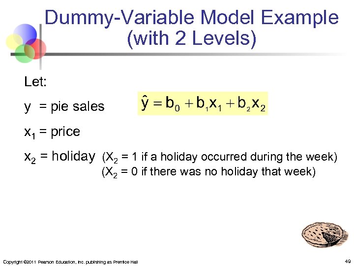
Dummy-Variable Model Example (with 2 Levels) Let: y = pie sales x 1 = price x 2 = holiday (X 2 = 1 if a holiday occurred during the week) (X 2 = 0 if there was no holiday that week) Copyright © 2011 Pearson Education, Inc. publishing as Prentice Hall 49
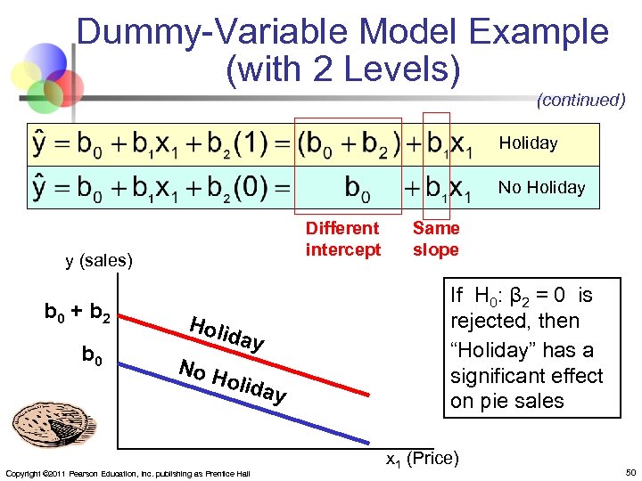
Dummy-Variable Model Example (with 2 Levels) (continued) Holiday No Holiday Different intercept y (sales) b 0 + b 2 b 0 Holi da y No H o liday Copyright © 2011 Pearson Education, Inc. publishing as Prentice Hall Same slope If H 0: β 2 = 0 is rejected, then “Holiday” has a significant effect on pie sales x 1 (Price) 50
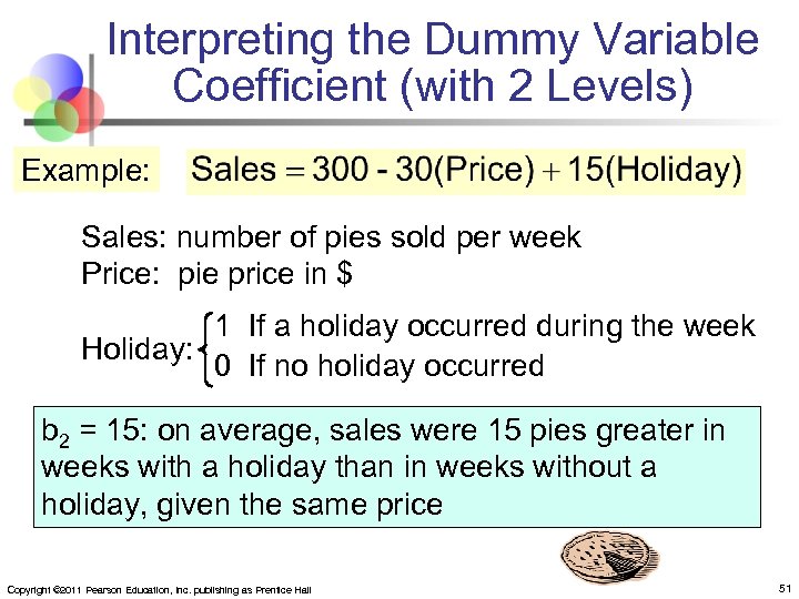
Interpreting the Dummy Variable Coefficient (with 2 Levels) Example: Sales: number of pies sold per week Price: pie price in $ 1 If a holiday occurred during the week Holiday: 0 If no holiday occurred b 2 = 15: on average, sales were 15 pies greater in weeks with a holiday than in weeks without a holiday, given the same price Copyright © 2011 Pearson Education, Inc. publishing as Prentice Hall 51
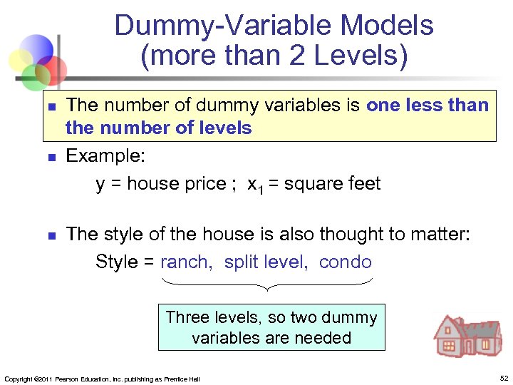
Dummy-Variable Models (more than 2 Levels) n n n The number of dummy variables is one less than the number of levels Example: y = house price ; x 1 = square feet The style of the house is also thought to matter: Style = ranch, split level, condo Three levels, so two dummy variables are needed Copyright © 2011 Pearson Education, Inc. publishing as Prentice Hall 52
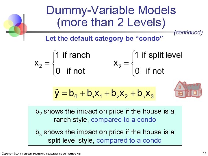
Dummy-Variable Models (more than 2 Levels) Let the default category be “condo” (continued) b 2 shows the impact on price if the house is a ranch style, compared to a condo b 3 shows the impact on price if the house is a split level style, compared to a condo Copyright © 2011 Pearson Education, Inc. publishing as Prentice Hall 53
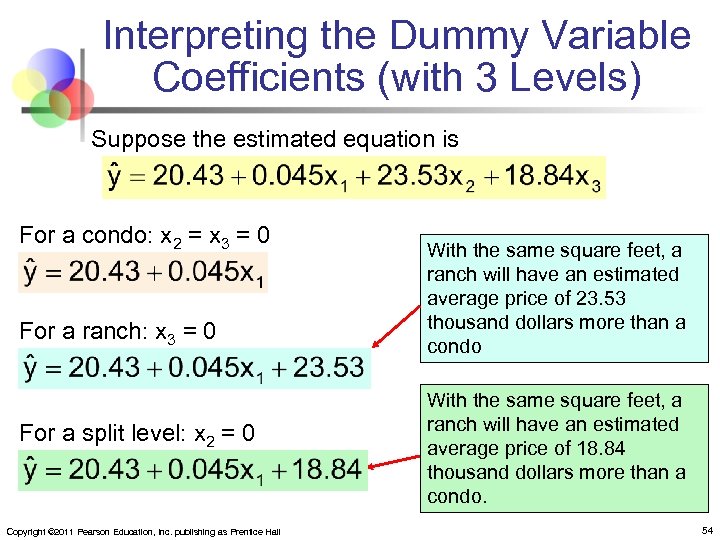
Interpreting the Dummy Variable Coefficients (with 3 Levels) Suppose the estimated equation is For a condo: x 2 = x 3 = 0 For a ranch: x 3 = 0 For a split level: x 2 = 0 Copyright © 2011 Pearson Education, Inc. publishing as Prentice Hall With the same square feet, a ranch will have an estimated average price of 23. 53 thousand dollars more than a condo With the same square feet, a ranch will have an estimated average price of 18. 84 thousand dollars more than a condo. 54
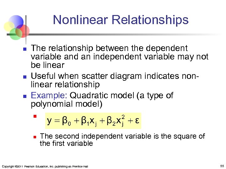
Nonlinear Relationships n n n The relationship between the dependent variable and an independent variable may not be linear Useful when scatter diagram indicates nonlinear relationship Example: Quadratic model (a type of polynomial model) n n The second independent variable is the square of the first variable Copyright © 2011 Pearson Education, Inc. publishing as Prentice Hall 55
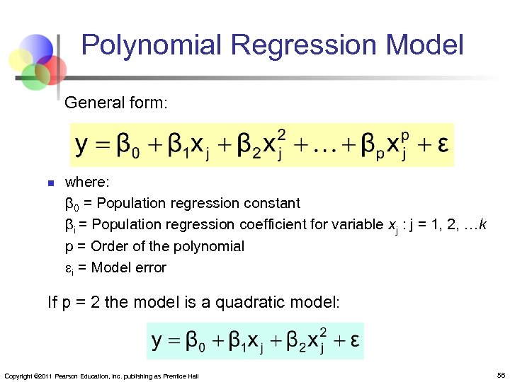
Polynomial Regression Model General form: n where: β 0 = Population regression constant βi = Population regression coefficient for variable xj : j = 1, 2, …k p = Order of the polynomial i = Model error If p = 2 the model is a quadratic model: Copyright © 2011 Pearson Education, Inc. publishing as Prentice Hall 56
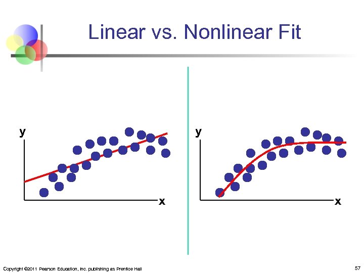
Linear vs. Nonlinear Fit y y x Copyright © 2011 Pearson Education, Inc. publishing as Prentice Hall x 57
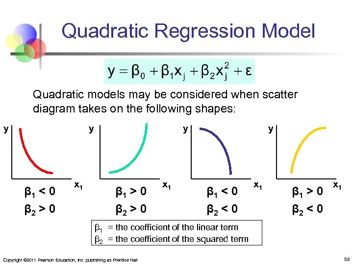
Quadratic Regression Model Quadratic models may be considered when scatter diagram takes on the following shapes: y y β 1 < 0 β 2 > 0 x 1 y β 1 > 0 β 2 > 0 x 1 y β 1 < 0 β 2 < 0 x 1 β 1 > 0 β 2 < 0 x 1 β 1 = the coefficient of the linear term β 2 = the coefficient of the squared term Copyright © 2011 Pearson Education, Inc. publishing as Prentice Hall 58
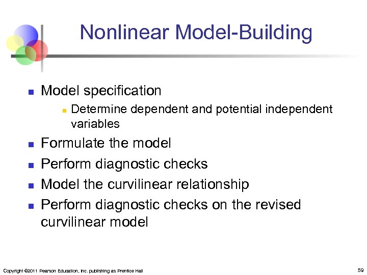
Nonlinear Model-Building n Model specification n n Determine dependent and potential independent variables Formulate the model Perform diagnostic checks Model the curvilinear relationship Perform diagnostic checks on the revised curvilinear model Copyright © 2011 Pearson Education, Inc. publishing as Prentice Hall 59
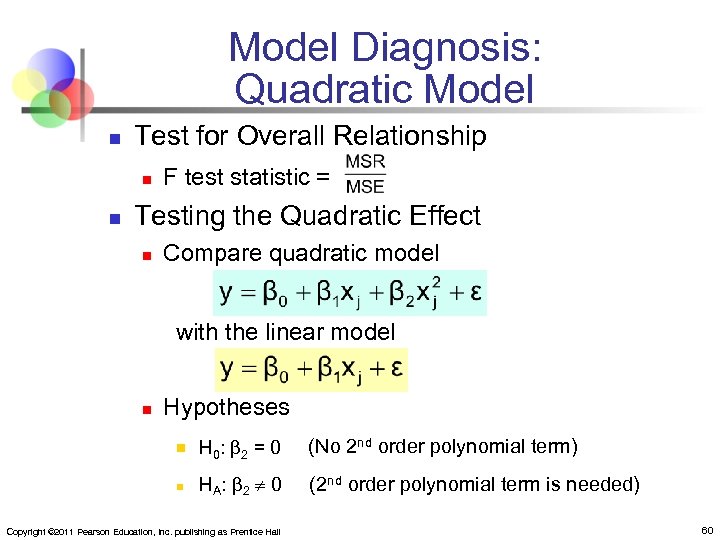
Model Diagnosis: Quadratic Model n Test for Overall Relationship n n F test statistic = Testing the Quadratic Effect n Compare quadratic model with the linear model n Hypotheses n H 0 : β 2 = 0 (No 2 nd order polynomial term) n HA : β 2 0 (2 nd order polynomial term is needed) Copyright © 2011 Pearson Education, Inc. publishing as Prentice Hall 60
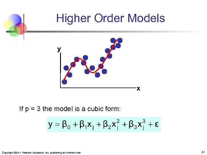
Higher Order Models y x If p = 3 the model is a cubic form: Copyright © 2011 Pearson Education, Inc. publishing as Prentice Hall 61
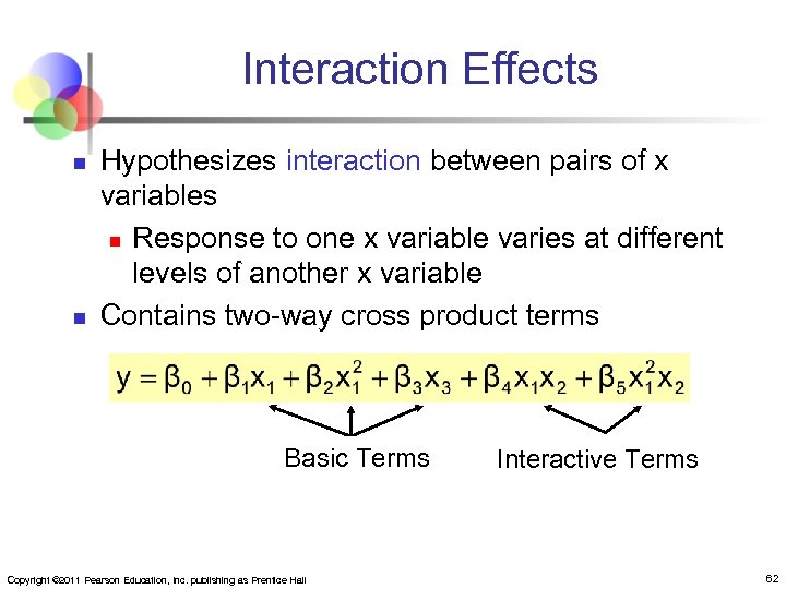
Interaction Effects n n Hypothesizes interaction between pairs of x variables n Response to one x variable varies at different levels of another x variable Contains two-way cross product terms Basic Terms Copyright © 2011 Pearson Education, Inc. publishing as Prentice Hall Interactive Terms 62
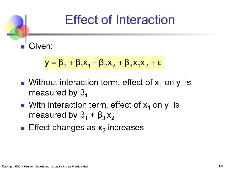
Effect of Interaction n n Given: Without interaction term, effect of x 1 on y is measured by β 1 With interaction term, effect of x 1 on y is measured by β 1 + β 3 x 2 Effect changes as x 2 increases Copyright © 2011 Pearson Education, Inc. publishing as Prentice Hall 63
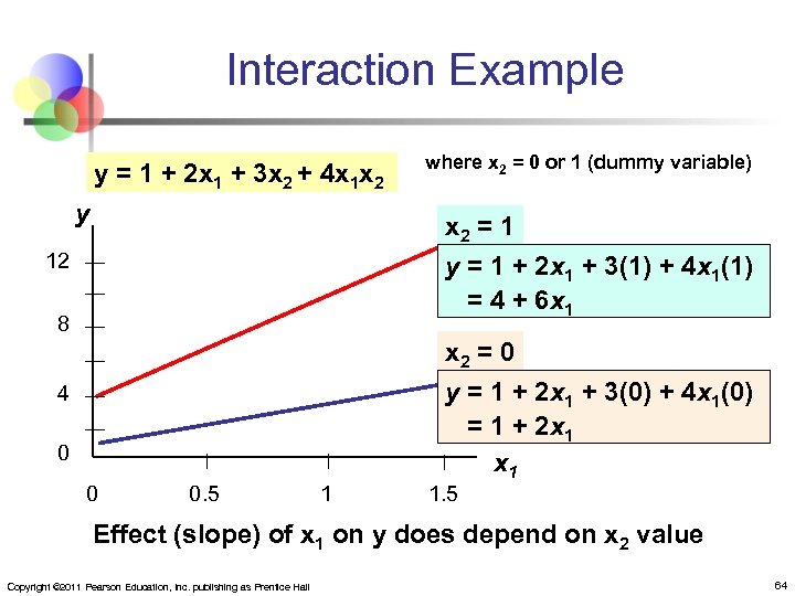
Interaction Example y = 1 + 2 x 1 + 3 x 2 + 4 x 1 x 2 y where x 2 = 0 or 1 (dummy variable) x 2 = 1 y = 1 + 2 x 1 + 3(1) + 4 x 1(1) = 4 + 6 x 1 12 8 4 0 0 0. 5 1 x 2 = 0 y = 1 + 2 x 1 + 3(0) + 4 x 1(0) = 1 + 2 x 1 1. 5 Effect (slope) of x 1 on y does depend on x 2 value Copyright © 2011 Pearson Education, Inc. publishing as Prentice Hall 64
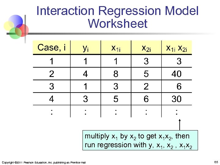
Interaction Regression Model Worksheet multiply x 1 by x 2 to get x 1 x 2, then run regression with y, x 1, x 2 , x 1 x 2 Copyright © 2011 Pearson Education, Inc. publishing as Prentice Hall 65
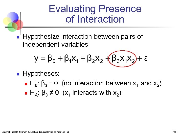
Evaluating Presence of Interaction n n Hypothesize interaction between pairs of independent variables Hypotheses: n H 0: β 3 = 0 (no interaction between x 1 and x 2) n HA: β 3 ≠ 0 (x 1 interacts with x 2) Copyright © 2011 Pearson Education, Inc. publishing as Prentice Hall 66
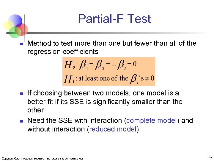
Partial-F Test n n n Method to test more than one but fewer than all of the regression coefficients If choosing between two models, one model is a better fit if its SSE is significantly smaller than the other Need the SSE with interaction (complete model) and without interaction (reduced model) Copyright © 2011 Pearson Education, Inc. publishing as Prentice Hall 67
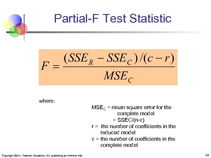
Partial-F Test Statistic where: MSEC = mean square error for the complete model = SSEC/(n-c) r = the number of coefficients in the reduced model c = the number of coefficients in the complete model Copyright © 2011 Pearson Education, Inc. publishing as Prentice Hall 68
Model Building n Goal is to develop a model with the best set of independent variables n n n Stepwise regression procedure n n Easier to interpret if unimportant variables are removed Lower probability of collinearity Provide evaluation of alternative models as variables are added Best-subset approach n Try all combinations and select the best using the highest adjusted R 2 and lowest sε Copyright © 2011 Pearson Education, Inc. publishing as Prentice Hall 69
Stepwise Regression n n Idea: develop the least squares regression equation in steps, either through forward selection, backward elimination, or through standard stepwise regression The Coefficient of Partial Determination is the measure of the marginal contribution of each independent variable, given that other independent variables are in the model Copyright © 2011 Pearson Education, Inc. publishing as Prentice Hall 70
Best Subsets Regression n Idea: estimate all possible regression equations using all possible combinations of independent variables Select subsets from the chose possible independent variables to form models Choose the best fit by looking for the highest adjusted R 2 and lowest standard error sε Stepwise regression and best subsets regression can be performed using PHStat, Minitab, or other statistical software packages Copyright © 2011 Pearson Education, Inc. publishing as Prentice Hall 71
Model Diagnosis: Aptness of the Model n Diagnostic checks on the model include verifying the assumptions of multiple regression: n Individual model errors are independent and random n Error are normally distributed n Errors have constant variance n Each xi is linearly related to y Errors (or Residuals) are given by Copyright © 2011 Pearson Education, Inc. publishing as Prentice Hall 72
Residual Analysis n Analysis of residuals can reveal: n n A nonlinear regression function Residuals that do not have a constant variance Residuals that are non independent Residual terms that are not normally distributed Copyright © 2011 Pearson Education, Inc. publishing as Prentice Hall 73
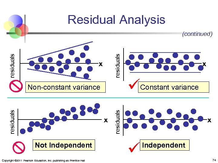
Residual Analysis residuals (continued) x x Not Independent Copyright © 2011 Pearson Education, Inc. publishing as Prentice Hall Constant variance residuals Non-constant variance x x Independent 74
The Normality Assumption n Errors are assumed to be normally distributed Standardized residuals can be calculated by computer Examine a histogram or a normal probability plot of the standardized residuals to check for normality Copyright © 2011 Pearson Education, Inc. publishing as Prentice Hall 75
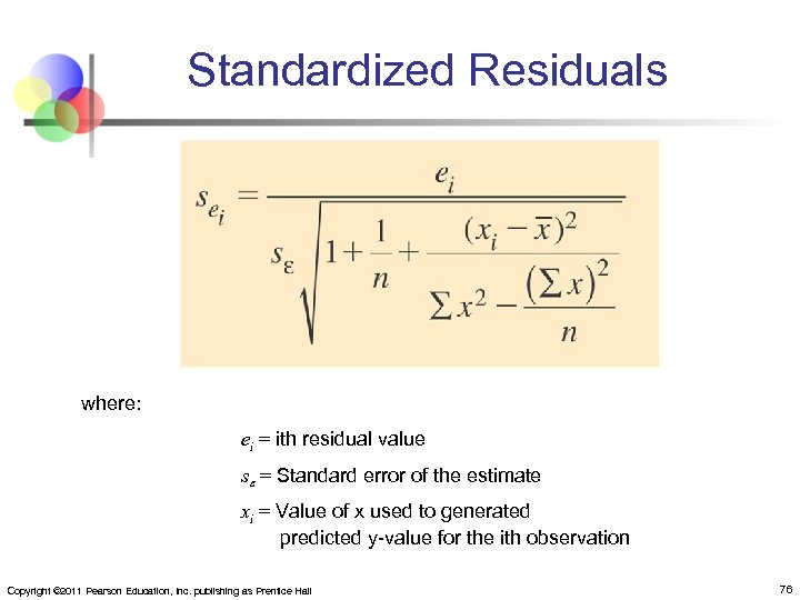
Standardized Residuals where: ei = ith residual value se = Standard error of the estimate xi = Value of x used to generated predicted y-value for the ith observation Copyright © 2011 Pearson Education, Inc. publishing as Prentice Hall 76
Corrective Actions n 3 approaches if the model is not appropriate: n Transform some of the independent variables (x) n n Raising x to a power Taking the square root of x Taking the log of x If the normality assumption is not met, transforming the dependent variable (y) may help also n Remove some variables from the model n Start over Copyright © 2011 Pearson Education, Inc. publishing as Prentice Hall 77
Chapter Summary n n n Developed the multiple regression model Tested the significance of the multiple regression model Developed adjusted R 2 Tested individual regression coefficients Used dummy variables Examined interaction in a multiple regression model Copyright © 2011 Pearson Education, Inc. publishing as Prentice Hall 78
Chapter Summary (continued) n n n Described nonlinear regression models Described multicollinearity Discussed model building n n n Stepwise regression Best subsets regression Examined residual plots to check model assumptions Copyright © 2011 Pearson Education, Inc. publishing as Prentice Hall 79

All rights reserved. No part of this publication may be reproduced, stored in a retrieval system, or transmitted, in any form or by any means, electronic, mechanical, photocopying, recording, or otherwise, without the prior written permission of the publisher. Printed in the United States of America. Copyright © 2011 Pearson Education, Inc. publishing as Prentice Hall 80
a56bc04cb42997f8dfbedcf82f64d1c9.ppt