Building VAR Models To find a VAR model

Building VAR Models To find a VAR model for time series TS 1, TS 2, TS 3, load them in Eviews and select “Estimate VAR…” from Quick menu. In the “Endogenous Variables” box type the names of variables: TS 1 TS 2 TS 3. The box “Lag Intervals for Endogenous” specifies the lags used in the VAR model. The default specification “ 1 2” means that two lags will be used for each endogenous variable.

Once you are happy with VAR Specifications press OK. A new window “Vector Autoregression Estimates” opens. It shows the values of parameters estimated for the specified VAR model and various summary statistics. The results are presented in three columns, TS 1 TS 2 TS 3, containing the estimates of the coefficients for all lagged endogenous variables, standard errors in ( ), and tstatistics in [ ], as well as the estimates of additive constants for each endogenous variable.

To select the best VAR model perform estimations for different lag specifications. For instance from “ 1 1” to “ 1 7” and choose the one with the minimal value of the Bayesian Schwarz Criterion for the entire system.

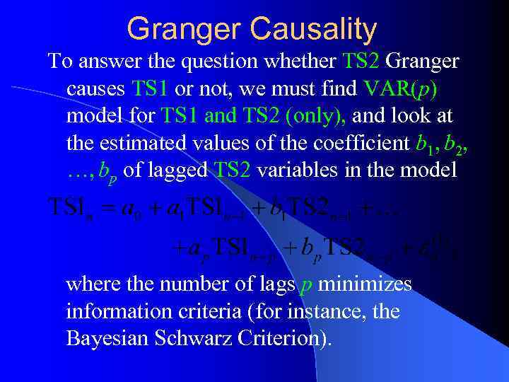
Granger Causality To answer the question whether TS 2 Granger causes TS 1 or not, we must find VAR(p) model for TS 1 and TS 2 (only), and look at the estimated values of the coefficient b 1, b 2, …, bp of lagged TS 2 variables in the model where the number of lags p minimizes information criteria (for instance, the Bayesian Schwarz Criterion).

If the value of at least one of the coefficients b 1, b 2, …, bp is outside the 95% confidence interval around 0 (that is, the value of the corresponding t-statistics is outside the interval [ – 1. 96, +1. 96]), then TS 2 Granger causes TS 1. If the t-statistics of all coefficients b 1, b 2, …, bp belong to the interval [ – 1. 96, +1. 96], then it is likely that TS 2 does not Granger causes TS 1. To obtain a more reliable conclusion in the latter case one has to run a joint test for the coefficients b 1, b 2, …, bp.

Click View in the VAR estimation window, then Lag Structure, and click Granger Causality. In the Granger Causality window find Dependent Variable: TS 1 and look at the line corresponding to the Excluded variable TS 2. If the Prob. Value is less than 0. 05 then TS 2 Granger causes TS 1 at the 5% confidence level. Otherwise TS 2 does not Granger cause TS 1 at the 5% confidence level.

Estimating TARCH(1, 1) Model Click Quick, then Estimate Equation. In the Equation specification window type the name of the dependent variable and the list of regressors. For instance, TS 3 c TS 3(-1) TS 3(-2) corresponds to the AR(2) – TARCH(1, 1) model. In the Estimation Setting box select Method: ARCH.

Equation Estimation window opens. Specify Threshold order: 1, and press OK. Equation output window opens. Find Variance Equation in the opened window, and look at the line RESID( -1)^2*(RESID(-1)<0) below. If the Prob. value in the line RESID(-1)^2*(RESID(-1)<0) is less than 0. 05, then the model is asymmetric (there is evidence of asymmetry). Otherwise, there is no evidence of asymmetry.

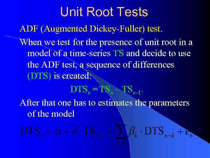
Unit Root Tests ADF (Augmented Dickey-Fuller) test. When we test for the presence of unit root in a model of a time-series TS and decide to use the ADF test, a sequence of differences (DTS) is created: DTSn = TSn – TSn-1. After that one has to estimates the parameters of the model

The number of lags h is the minimal integer number, such that the residual of the estimated model are uncorrelated. That is the values of the autocorrelation function belong to the 95% confidence intervals around 0. Actually, 5% of the values of the autocorrelation functions should lie outside the 95% confidence intervals. Therefore, to make a valid conclusion if the residual are uncorrelated or not, one can use statistical tests.

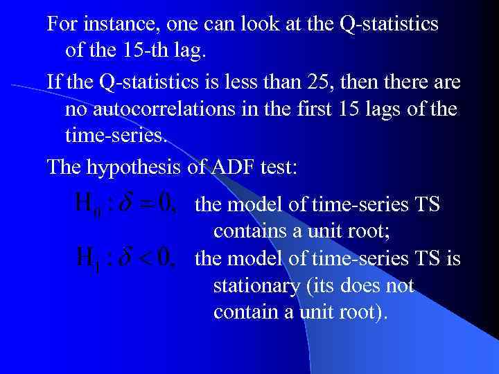
For instance, one can look at the Q-statistics of the 15 -th lag. If the Q-statistics is less than 25, then there are no autocorrelations in the first 15 lags of the time-series. The hypothesis of ADF test: the model of time-series TS contains a unit root; the model of time-series TS is stationary (its does not contain a unit root).

To run the ADF test in EViews, open (double click) the time series TS. Then click View, and choose Unit Root Test… Select Augmented Dickey-Fuller in the Test type box. EViews will try to choose the number of lags h automatically. However, if you are not happy with the automatic choice, you can supply the desired number of lags (select User specified). Press OK once you are happy with Unit Root

A window with ADF Unit Root Test results opens. Find the line Augmented Dickey-Fuller test statistic, and look for Prob. value. If the Prob value is greater than 0. 05, then the TS time-series contains a unit root. If the Prob value is less than 0. 05, then the TS time series is stationary (it does not contain a unit root). The ARIMA model for the time series TS is ARIMA(p, 0, q) = ARMA(p, q).

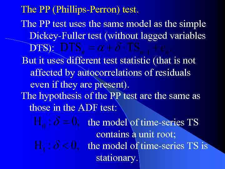
The PP (Phillips-Perron) test. The PP test uses the same model as the simple Dickey-Fuller test (without lagged variables DTS): But it uses different test statistic (that is not affected by autocorrelations of residuals even if they are present). The hypothesis of the PP test are the same as those in the ADF test: the model of time-series TS contains a unit root; the model of time-series TS is stationary.

To run the PP test in EViews, open (double click) the time series TS. Then click View, and choose Unit Root Test… Select Phillips-Perron in the Test type box, and press OK

A window with PP Unit Root Test results opens. Find the line Phillips-Perron test statistic, and look for Prob. value. If the Prob value is greater than 0. 05, then the TS time-series contains a unit root. If the Prob value is less than 0. 05, then the TS time series is stationary (it does not contain a unit root). The ARIMA model for the time series TS is ARIMA(p, 0, q) = ARMA(p, q).

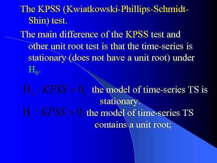
The KPSS (Kwiatkowski-Phillips-Schmidt. Shin) test. The main difference of the KPSS test and other unit root test is that the time-series is stationary (does not have a unit root) under H 0. the model of time-series TS is stationary. the model of time-series TS contains a unit root;

To run the KPSS test in EViews, open (double click) the time series TS. Then click View, and choose Unit Root Test… Select Kwiatkowski-Phillips-Schmidt-Shin in the Test type box, and press OK.

A window with KPSS Unit Root Test results opens. Find the line Kwiatkowski-Phillips-Schmidt. Shin test statistic, and look for LM-Stat value. If the LM-Stat value is less than 5% level value, then the TS time series is stationary (it does not contain a unit root). The ARIMA model for the time series TS is ARIMA(p, 0, q) = ARMA(p, q). If the LM-Stat value is greater than 5% level value, then the TS time series contains a unit root.

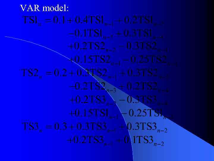
VAR model: