Building Statistical Forecast Models Wes Wilson MIT Lincoln

Building Statistical Forecast Models Wes Wilson MIT Lincoln Laboratory April, 2001 Stat. Fcst. Models Wes Wilson 3/15/2018 MIT Lincoln Laboratory

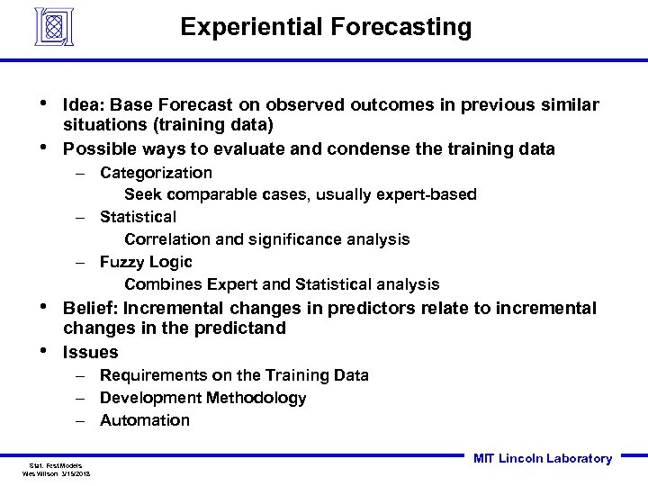
Experiential Forecasting • • Idea: Base Forecast on observed outcomes in previous similar situations (training data) Possible ways to evaluate and condense the training data – Categorization Seek comparable cases, usually expert-based – Statistical Correlation and significance analysis – Fuzzy Logic Combines Expert and Statistical analysis • • Belief: Incremental changes in predictors relate to incremental changes in the predictand Issues – Requirements on the Training Data – Development Methodology – Automation Stat. Fcst. Models Wes Wilson 3/15/2018 MIT Lincoln Laboratory

Outline • • • Regression-based Models Predictor Selection Data Quality and Clustering Measuring Success An Example Stat. Fcst. Models Wes Wilson 3/15/2018 MIT Lincoln Laboratory

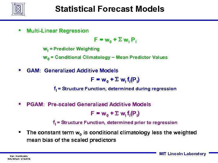
Statistical Forecast Models • Multi-Linear Regression F = w 0 + S wi P i wi = Predictor Weighting w 0 = Conditional Climatology Mean Predictor Values • GAM: Generalized Additive Models F = w 0 + S wi fi(Pi) fi = Structure Function, determined during regression • PGAM: Pre-scaled Generalized Additive Models F = w 0 + S wi fi(Pi) fi = Structure Function, determined prior to regression • The constant term w 0 is conditional climatology less the weighted mean bias of the scaled predictors Stat. Fcst. Models Wes Wilson 3/15/2018 MIT Lincoln Laboratory

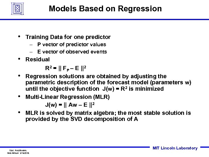
Models Based on Regression • Training Data for one predictor – P vector of predictor values – E vector of observed events • • Residual R 2 = || FP – E ||2 Regression solutions are obtained by adjusting the parametric description of the forecast model (parameters w) until the objective function J(w) = R 2 is minimized Multi-Linear Regression (MLR) J(w) = || Aw – E ||2 MLR is solved by matrix algebra; the most stable solution is provided by the SVD decomposition of A Stat. Fcst. Models Wes Wilson 3/15/2018 MIT Lincoln Laboratory

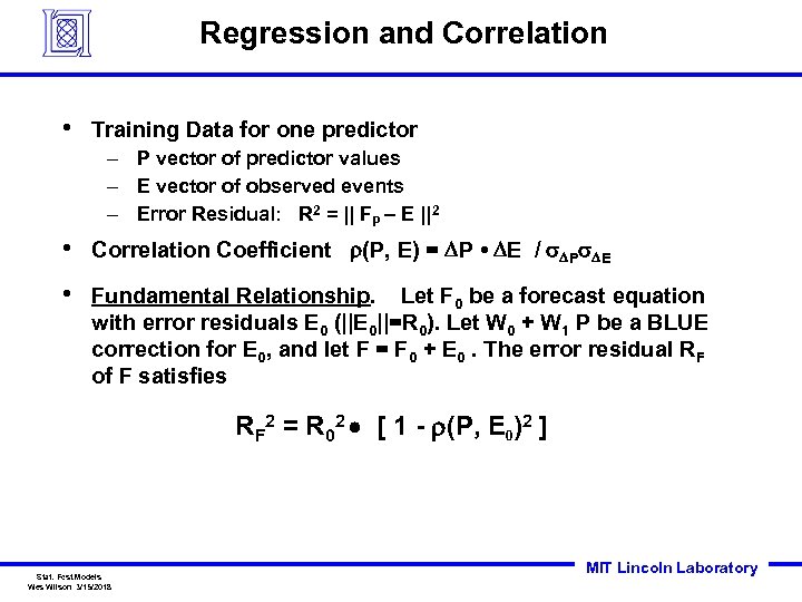
Regression and Correlation • Training Data for one predictor – P vector of predictor values – E vector of observed events – Error Residual: R 2 = || FP – E ||2 • Correlation Coefficient r(P, E) = DP • DE / s. DPs. DE • Fundamental Relationship. Let F 0 be a forecast equation with error residuals E 0 (||E 0||=R 0). Let W 0 + W 1 P be a BLUE correction for E 0, and let F = F 0 + E 0. The error residual RF of F satisfies RF 2 = R 02 [ 1 - r(P, E 0)2 ] Stat. Fcst. Models Wes Wilson 3/15/2018 MIT Lincoln Laboratory

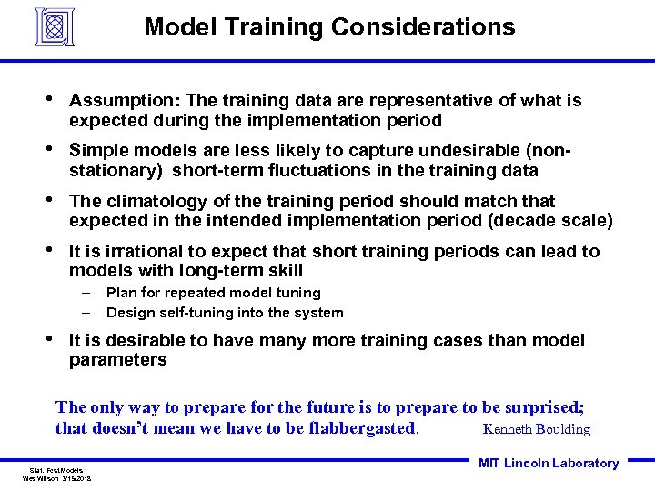
Model Training Considerations • Assumption: The training data are representative of what is expected during the implementation period • Simple models are less likely to capture undesirable (nonstationary) short-term fluctuations in the training data • The climatology of the training period should match that expected in the intended implementation period (decade scale) • It is irrational to expect that short training periods can lead to models with long-term skill – – • Plan for repeated model tuning Design self-tuning into the system It is desirable to have many more training cases than model parameters The only way to prepare for the future is to prepare to be surprised; that doesn’t mean we have to be flabbergasted. Kenneth Boulding Stat. Fcst. Models Wes Wilson 3/15/2018 MIT Lincoln Laboratory

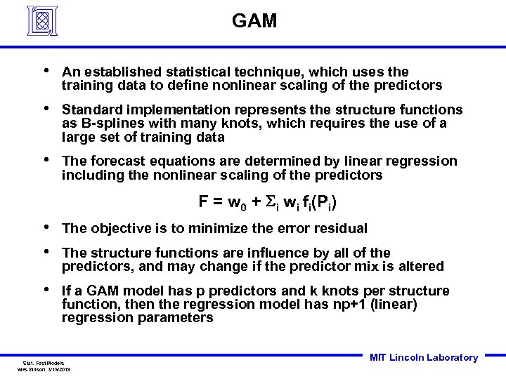
GAM • An established statistical technique, which uses the training data to define nonlinear scaling of the predictors • Standard implementation represents the structure functions as B-splines with many knots, which requires the use of a large set of training data • The forecast equations are determined by linear regression including the nonlinear scaling of the predictors F = w 0 + Si wi fi(Pi) • • The objective is to minimize the error residual • If a GAM model has p predictors and k knots per structure function, then the regression model has np+1 (linear) regression parameters The structure functions are influence by all of the predictors, and may change if the predictor mix is altered Stat. Fcst. Models Wes Wilson 3/15/2018 MIT Lincoln Laboratory

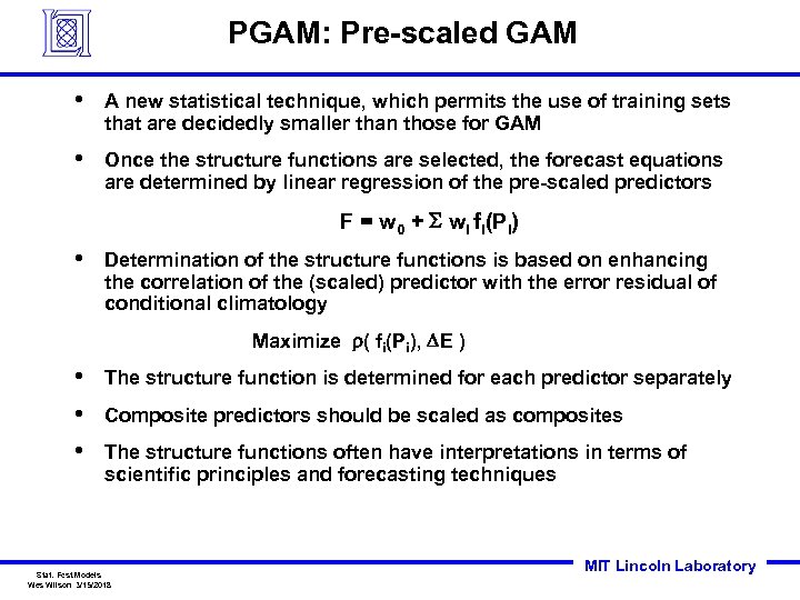
PGAM: Pre-scaled GAM • A new statistical technique, which permits the use of training sets that are decidedly smaller than those for GAM • Once the structure functions are selected, the forecast equations are determined by linear regression of the pre-scaled predictors F = w 0 + S wi fi(Pi) • Determination of the structure functions is based on enhancing the correlation of the (scaled) predictor with the error residual of conditional climatology Maximize r( fi(Pi), DE ) • • • The structure function is determined for each predictor separately Composite predictors should be scaled as composites The structure functions often have interpretations in terms of scientific principles and forecasting techniques Stat. Fcst. Models Wes Wilson 3/15/2018 MIT Lincoln Laboratory

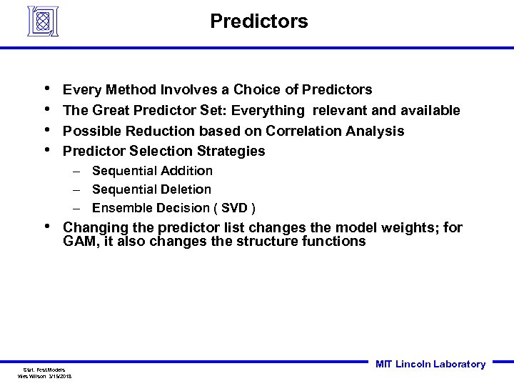
Predictors • • Every Method Involves a Choice of Predictors The Great Predictor Set: Everything relevant and available Possible Reduction based on Correlation Analysis Predictor Selection Strategies – Sequential Addition – Sequential Deletion – Ensemble Decision ( SVD ) • Changing the predictor list changes the model weights; for GAM, it also changes the structure functions Stat. Fcst. Models Wes Wilson 3/15/2018 MIT Lincoln Laboratory

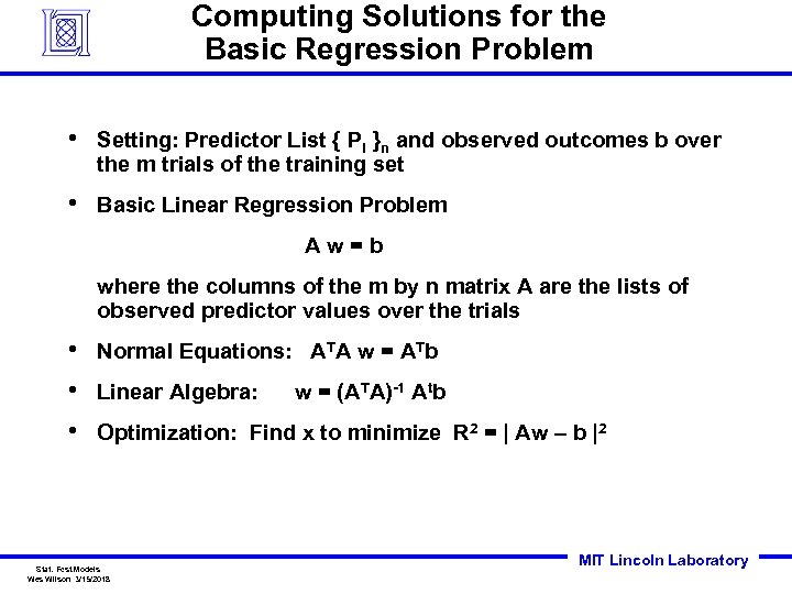
Computing Solutions for the Basic Regression Problem • Setting: Predictor List { Pi }n and observed outcomes b over the m trials of the training set • Basic Linear Regression Problem Aw=b where the columns of the m by n matrix A are the lists of observed predictor values over the trials • • • Normal Equations: ATA w = ATb Linear Algebra: w = (ATA)-1 Atb Optimization: Find x to minimize R 2 = | Aw – b |2 Stat. Fcst. Models Wes Wilson 3/15/2018 MIT Lincoln Laboratory

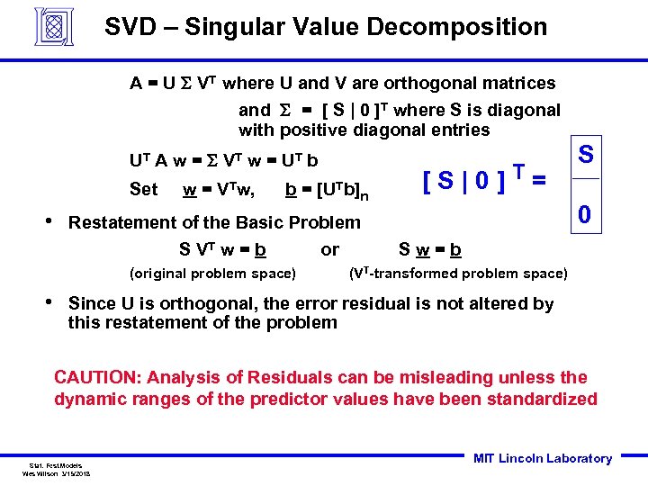
SVD – Singular Value Decomposition A = U S VT where U and V are orthogonal matrices and S = [ S | 0 ]T where S is diagonal with positive diagonal entries UT A w = S V T w = U T b Set • w= VTw, b= n Restatement of the Basic Problem S VT w = b or (original problem space) • [UTb] [S|0]T= S 0 Sw=b (VT-transformed problem space) Since U is orthogonal, the error residual is not altered by this restatement of the problem CAUTION: Analysis of Residuals can be misleading unless the dynamic ranges of the predictor values have been standardized Stat. Fcst. Models Wes Wilson 3/15/2018 MIT Lincoln Laboratory

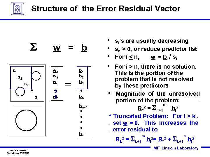
Structure of the Error Residual Vector S s 1 w = b w 1 w 2 w 3 s 2 s 3 * sn * 0 wn 0 = b 1 b 2 b 3 * bn si’s are usually decreasing sn > 0, or reduce predictor list For i < n, w i = b i / si For i > n, there is no solution. This is the portion of the problem that is not resolved by these predictors • Magnitude of the unresolved portion of the problem: m R*2 = Sn+1 bi 2 • Truncated Problem: For i > k , set wi = 0. This increases the error residual to . bn+1 * * bm Stat. Fcst. Models Wes Wilson 3/15/2018 • • . . Rk = Sk+1 2 m bi 2= R*2 n + Sk+1 bi 2 MIT Lincoln Laboratory

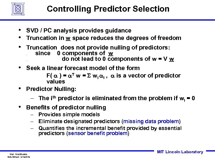
Controlling Predictor Selection • • • SVD / PC analysis provides guidance Truncation in w space reduces the degrees of freedom Truncation does not provide nulling of predictors: since 0 components of w do not lead to 0 components of w = V w. . • • Seek a linear forecast model of the form F( a ) = a. T w = S wi ai , a is a vector of predictor values Predictor Nulling: – The ith predictor is eliminated from the problem if wi = 0 • Benefits of predictor nulling – Provides simple models – Eliminate designated predictors (missing data problem) – Quantifies the incremental benefit provided by essential predictors (sensor benefit problem) Stat. Fcst. Models Wes Wilson 3/15/2018 MIT Lincoln Laboratory

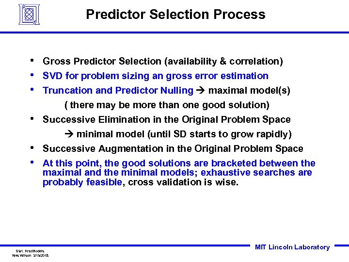
Predictor Selection Process • • • Gross Predictor Selection (availability & correlation) SVD for problem sizing an gross error estimation Truncation and Predictor Nulling maximal model(s) ( there may be more than one good solution) • Successive Elimination in the Original Problem Space minimal model (until SD starts to grow rapidly) • • Successive Augmentation in the Original Problem Space At this point, the good solutions are bracketed between the maximal and the minimal models; exhaustive searches are probably feasible, cross validation is wise. Stat. Fcst. Models Wes Wilson 3/15/2018 MIT Lincoln Laboratory

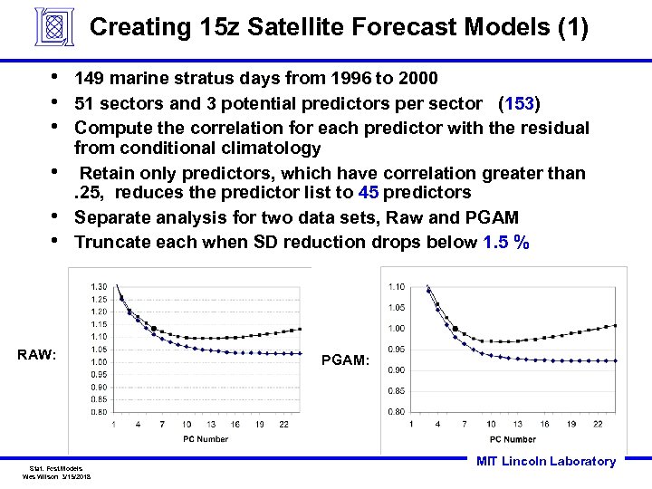
Creating 15 z Satellite Forecast Models (1) • • • 149 marine stratus days from 1996 to 2000 51 sectors and 3 potential predictors per sector (153) Compute the correlation for each predictor with the residual from conditional climatology Retain only predictors, which have correlation greater than. 25, reduces the predictor list to 45 predictors Separate analysis for two data sets, Raw and PGAM Truncate each when SD reduction drops below 1. 5 % RAW: Stat. Fcst. Models Wes Wilson 3/15/2018 PGAM: MIT Lincoln Laboratory

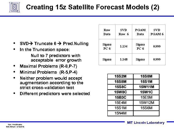
Creating 15 z Satellite Forecast Models (2) Raw Data • • • SVD Truncate 6 Pred. Nulling In the Truncation space: Null to 7 predictors with acceptable error growth Maximal Problems (R-8, P-7) Minimal Problems (R-5, P-4) Neither problem would accept augmentation according to the strict cross-validation test Different predictors were selected Stat. Fcst. Models Wes Wilson 3/15/2018 SVD Raw 6 PGAM Data SVD PGAM 6 Sigma PC 6 1. 134 Sigma PC 6 0. 999 Sigma 1. 148 Sigma 0. 999 MIT Lincoln Laboratory

Data Quality and Clustering • DQA is similar to NWP – need to do the training set – probably need to work to tighter standards • Data Clustering – During training - manual ++ – For implementation - fully automated • Conditional Climatology based on Clustering Stat. Fcst. Models Wes Wilson 3/15/2018 MIT Lincoln Laboratory

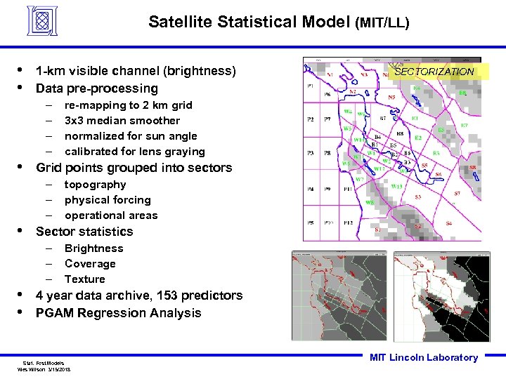
Satellite Statistical Model (MIT/LL) • • 1 -km visible channel (brightness) Data pre-processing – – • topography physical forcing operational areas Sector statistics – – – • • re-mapping to 2 km grid 3 x 3 median smoother normalized for sun angle calibrated for lens graying Grid points grouped into sectors – – – • SECTORIZATION Brightness Coverage Texture 4 year data archive, 153 predictors PGAM Regression Analysis Stat. Fcst. Models Wes Wilson 3/15/2018 MIT Lincoln Laboratory

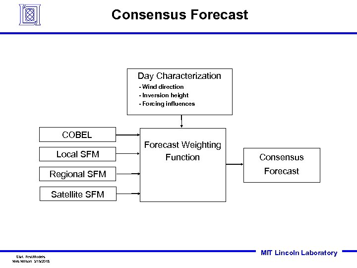
Consensus Forecast Day Characterization - Wind direction - Inversion height - Forcing influences COBEL Local SFM Regional SFM Forecast Weighting Function Consensus Forecast Satellite SFM Stat. Fcst. Models Wes Wilson 3/15/2018 MIT Lincoln Laboratory

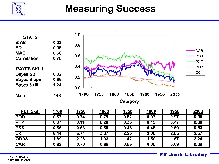
Measuring Success Stat. Fcst. Models Wes Wilson 3/15/2018 MIT Lincoln Laboratory

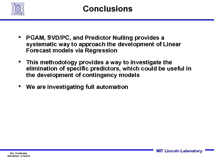
Conclusions • PGAM, SVD/PC, and Predictor Nulling provides a systematic way to approach the development of Linear Forecast models via Regression • This methodology provides a way to investigate the elimination of specific predictors, which could be useful in the development of contingency models • We are investigating full automation Stat. Fcst. Models Wes Wilson 3/15/2018 MIT Lincoln Laboratory