b1aea55848b2e299e70f400bd5302de9.ppt
- Количество слайдов: 45

Boolean + Ranking: Querying a Database by K-Constrained Optimization Zhen Zhang Seung-won Hwang Kevin C. Chang Min Wang Christian A. Lang Yuan-chi Chang Presented ACM SIGMOD Conference (SIGMOD 2006), Chicago, June 2006 Presented By : Pavan Kumar M. K. (1000618890) Aditya Mangipudi (1000649172)

Outline Introduction Motivation A* Search Algorithm A*-Driven State Space Construction Optimization Driven Configuration OPT* Search Algorithm Experiments Conclusion
Motivation The wide spread of databases for managing structured data, compounded with the expanded reach of the Internet, has brought forward interesting data retrieval and analysis scenarios to RDBMS Only the Top-K results are of interest to the user.

K-Constrained Optimization Query QUERY: Select the Top-5 2 nd year students in CSE with highest GPA Boolean query: Qualifying constraint dept = CSE and year = 2 + Ranking query: Top 5 ranked by GPA Find top answers B: dept = CSE and year = 2 O: GPA Quantifying function 4
K-Constrained Optimization Query Q = (G, k) G - Goal Function G=B. O k – Retrieval Size
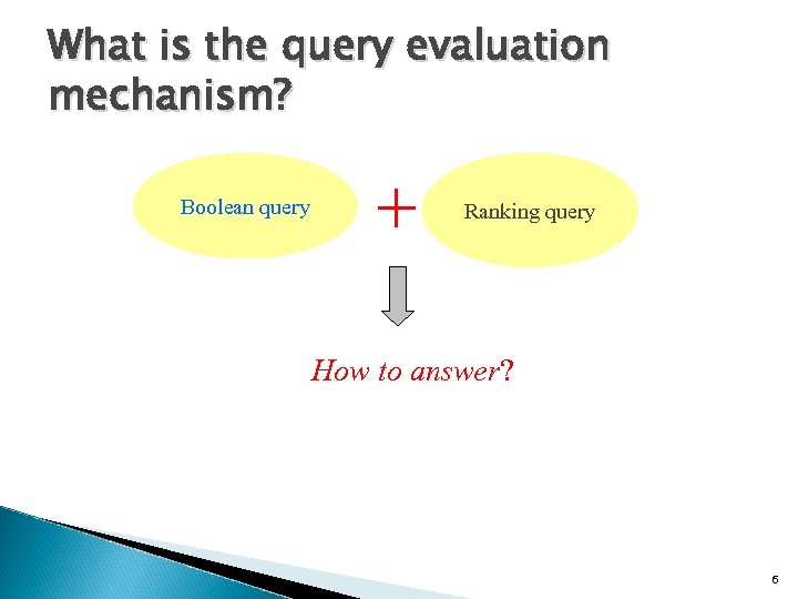
What is the query evaluation mechanism? Boolean query + Ranking query How to answer? 6
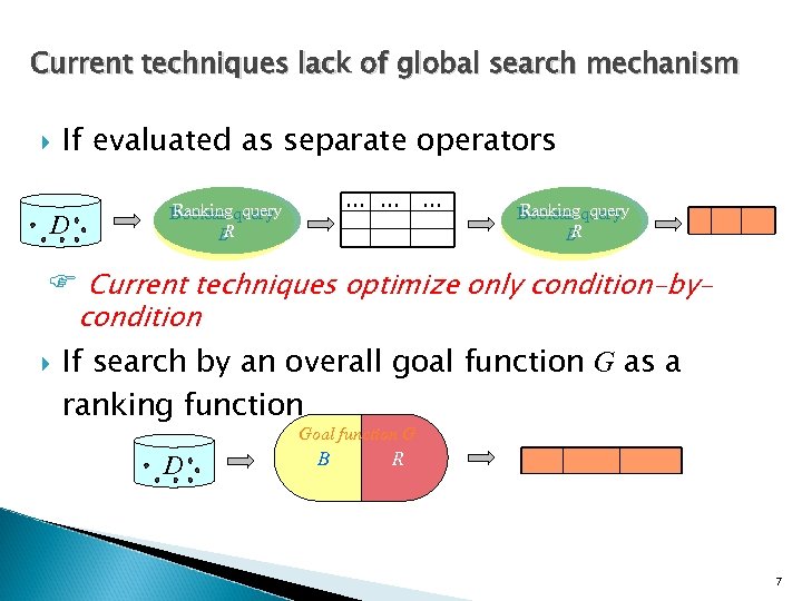
Current techniques lack of global search mechanism If evaluated as separate operators D … … Ranking query Boolean query R B F Current techniques optimize only condition-bycondition If search by an overall goal function G as a ranking function Goal function G D B R 7
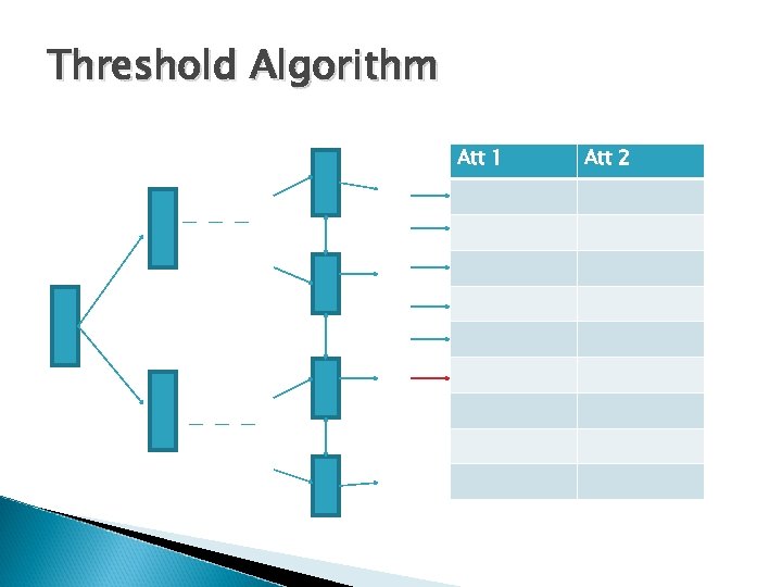
Threshold Algorithm Att 1 Att 2
Assumptions Threshold Algorithm essentially relies on a rigid assumption that G functions are Monotonic. The monotonicity requires G to be decreasing if all its parameters are decreasing.
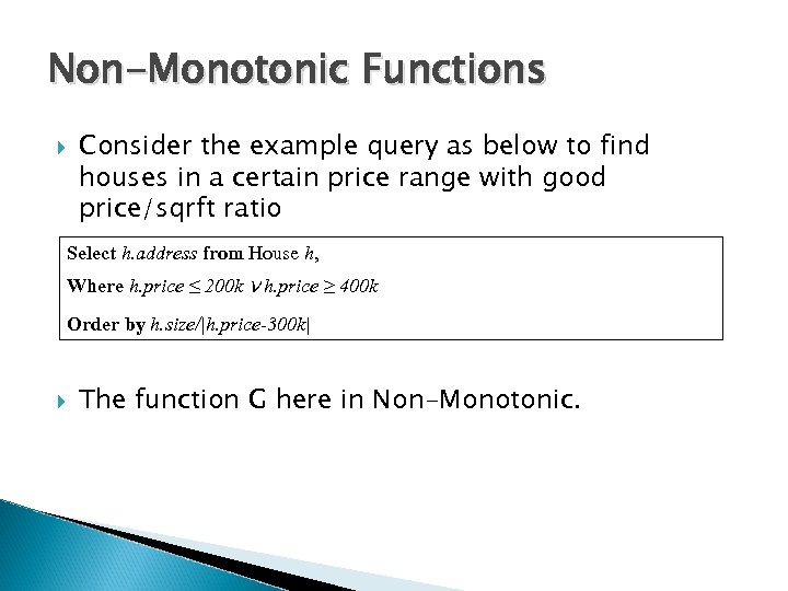
Non-Monotonic Functions Consider the example query as below to find houses in a certain price range with good price/sqrft ratio Select h. address from House h, Where h. price ≤ 200 k ν h. price ≥ 400 k Order by h. size/|h. price-300 k| The function G here in Non-Monotonic.

New Algorithm Att 1 Att 2
Need for encoding as a search problem Existing algorithms build upon their problemspecific assumptions on the goal functions or index traversals. For example, Threshold Algorithm assumes the monotonicity of G and the use of sorted accesses (interleaf navigation), based on which the search is implicitly hardwired. In a Boolean Query like B = price > 100 K, such a search is straightforward as the constraint expressions B explicitly suggests how to carry out a focused search, eg. , visiting only the nodes with locality potentially satisfying B.
Need for encoding as a search problem In contrast, for a general k-constrained optimization query potentially involving arbitrary ranking combined with Boolean conditions and joining multiple relations, eg. . Q maximizing size/price ratio, it is no longer clear how to focus the search. By encoding into a generic search with no assumptions on G, the search is generalized to support arbitrary G over potentially multiple indices and a combination of both hierarchical and interleaf traversals.
A* Algorithm A* is a well known search algorithm that finds the Shortest Path, given an initial and a designated goal state. Widely used in the field of Artificial Intelligence. Uses Best-First Search Traversal. Uses heuristic information to carry out the search in a guided manner. A* is guaranteed to find the correct answer (Correctness) by visiting the least number of states (Optimality) Ex: GPS, Google Maps, A lot of puzzles, games etc.
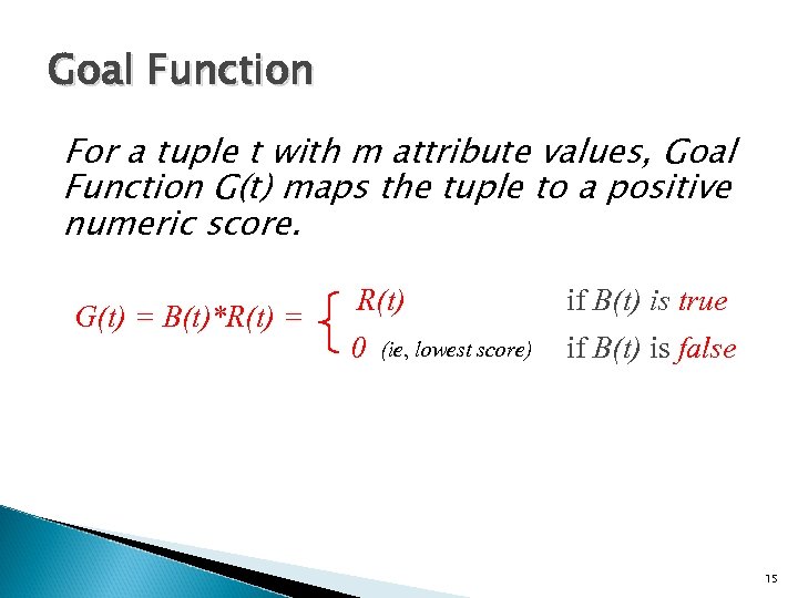
Goal Function For a tuple t with m attribute values, Goal Function G(t) maps the tuple to a positive numeric score. G(t) = B(t)*R(t) = R(t) if B(t) is true 0 if B(t) is false (ie, lowest score) 15

Query Model Addr Price Size Score 1. Oak park, Chicago 600 K 4500 15 Where h. price ≤ 200 k ν h. price ≥ 400 k 2. Mattis, Champaign 350 K 2000 0 Order by h. size/|h. price-300 k| 3. … 150 K 1000 6. 67 4. … 250 K 2000 0 5. … 300 K 3500 0 6. … 80 K 500 2. 27 Select h. address from House h,

Landscape of Score Function - G Addr Price Size Score 1. Oak park, Chicago 600 K 4500 15 2. Mattis, Champaign 350 K 2000 0 3. … 150 K 1000 6. 67 4. … 250 K 2000 0 5. … 300 K 3500 0 6. … 80 K 500 2. 27

OPT* Framework To realize k-constrained optimization over databases, this paper develops the OPT* framework. Objective: To Optimize G with the help of indices as access methods over tuples in D. Discrete State Search: From the view of using indices, we are to search the maximizing tuples on the index nodes as “discrete states”. Continuous Function Optimization: From the view of maximizing goal functions, we are to optimize G.
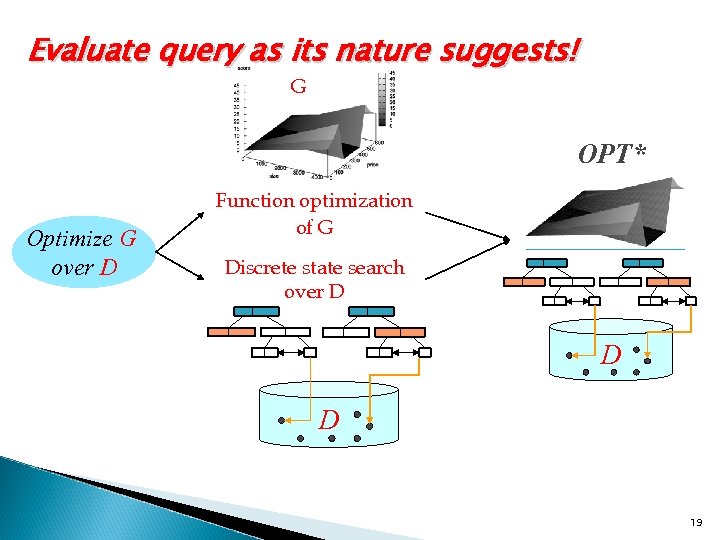
Evaluate query as its nature suggests! G OPT* Optimize G over D Function optimization of G Discrete state search over D D D 19

B+ Tree Structure Indices Value Space

Some definitions first. . States : States in a search graph represent “localities” of values at different granularity– from coarse to fine, and eventually reach tuples in the database. • Region State • Tuple State Transitions : While states of space give “locations” in the map, transitions further capture possible paths followed to reach our destination of query answers. Example : for two states u and v, there is a transition (u, v) if v ∈ Next(u)
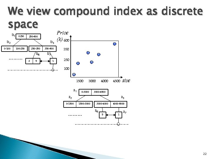
We view compound index as discrete space b 1 0 -250 250 -600 b 2 0 -100 b 3 100 -250 ……… 250 -350 b 6 2 5 350 -600 b 7 1 Price (k) 600 1 350 2 250 5 4 3 100 6 1500 a 1 3000 0 -3000 4500 3000 -4500 a 2 0 -1500 size a 3 1500 -3000 ……… 3000 -4000 a 6 5 4000 -6000 1 a 7 22
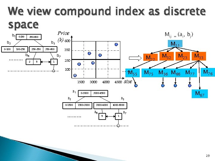
We view compound index as discrete space b 1 250 -600 0 -250 b 2 0 -100 b 3 100 -250 ……… 250 -350 b 7 5 1 Mij 2 250 5 M 22 4 3 …… M 100 55 6 1500 a 1 0 -3000 4000 4500 size 3000 -4500 a 2 0 -1500 a 3 1500 -3000 ……… 3000 -4000 a 6 5 = (ai, bj) M 11 1 350 -600 b 6 2 Price (k) 600 4 M 32 M 23 M 33 M 75 M 56 M 66 M 77 2 5 M 76 1 M 67 4000 -6000 1 a 7 23

We view compound index as discrete conceptually, combined space b 1 0 -250 250 -600 b 2 0 -100 b 3 100 -250 ……… 250 -350 Price (k) 600 b 7 5 2 250 1 5 M 22 M 32 M 23 M 33 4 3 100 … M 55 M 75 M 56 M 66 M 77 M 67 M 76 6 1500 a 1 0 -3000 4000 4500 size 4 2 5 1 3000 -4500 a 2 0 -1500 M 11 1 350 -600 b 6 2 Mij =(ai, bj) a 3 1500 -3000 ……… 3000 -4000 a 6 5 4000 -6000 1 a 7 24

Challenge 1: What is the search mechanism? 25

Encoding the problem into shortest path is challenging K-constrained optimization A* Shortest path Find a tuple with maximal score Find a path with minimal distance > A* Gives Shortest Path to testable goal. > The goal is to find optimal tuple states with maximal G-Score. 26
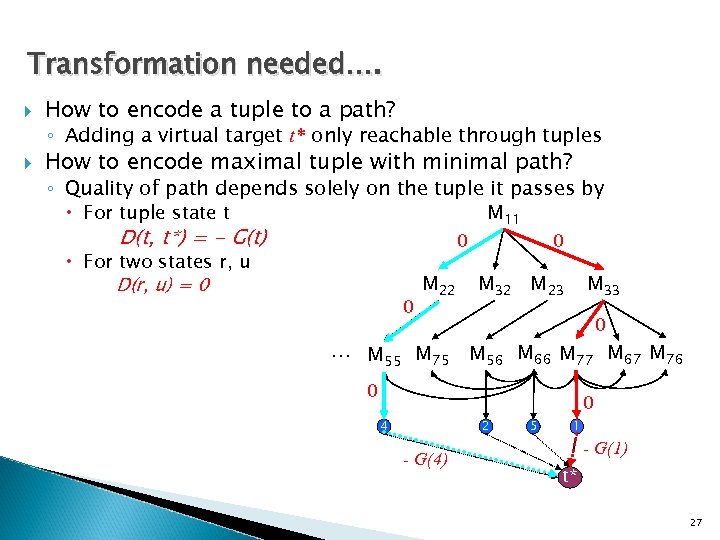
Transformation needed…. How to encode a tuple to a path? ◦ Adding a virtual target t* only reachable through tuples How to encode maximal tuple with minimal path? ◦ Quality of path depends solely on the tuple it passes by M 11 For tuple state t D(t, t*) = - G(t) 0 0 For two states r, u M 22 M 32 M 23 M 33 D(r, u) = 0 0 … M 55 M 75 0 M 56 M 66 M 77 M 67 M 76 0 4 2 - G(4) 5 1 0 - G(1) t* 27

Challenge 2: How to guide the search? 28

Functional Optimization perspective… Function optimization measures quality of states Function optimization aspects: • Defines Proper Heuristics • Identifies a set of initial states to start search. 29

Structure of Procedure OPT Input : G(x 1, ……, xm) and domain of values dom = xi ε [xi 1, xi 2] Output : <O, U> = OPT(G, dom) where O={gives local optima} U={Upper Bound Score} OPTPOINT gives O Component of OPTMAX gives U Component of OPT Approaches ØAnalytical Method ØSeach based (Ex: Hill Climbing) ØTemplate Based
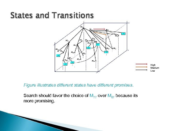
States and Transitions High Medium Low Figure illustrates different states have different promises. Search should favor the choice of M 77 over M 67 because its more promising.
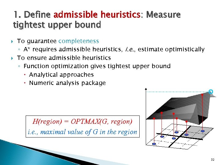
1. Define admissible heuristics: Measure tightest upper bound To guarantee completeness ◦ A* requires admissible heuristics, i. e. , estimate optimistically To ensure admissible heuristics ◦ Function optimization gives tightest upper bound Analytical approaches Numeric analysis package H(region) = OPTMAX(G, region) i. e. , maximal value of G in the region 32
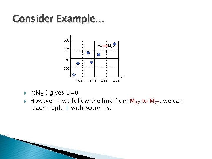
Consider Example… 600 M 67 350 2 250 3 M 77 1 5 4 100 6 1500 3000 4500 h(M 67) gives U=0 However if we follow the link from M 67 to M 77, we can reach Tuple 1 with score 15.

2. Configure descending space: disconnect uphills To guarantee optimality ◦ A* requires descending heuristics To ensure descending heuristics ◦ Remove uphill links M 11 M 22 M 32 M 23 M 33 … M 55 M 75 M 56 M 66 4 2 5 M 77 M 67 M 76 1 34
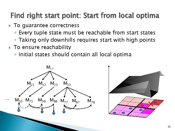
Find right start point: Start from local optima To guarantee correctness ◦ Every tuple state must be reachable from start states ◦ Taking only downhills requires start with high points To ensure reachability ◦ Initial states should contain all local optima M 11 M 22 M 32 M 23 … M 55 M 75 4 M 33 M 56 M 66 M 77 M 67 2 5 M 76 1 35

Putting together: Executing A* on the configured space top-down M 11 M 22 … M 55 4 n M 75 M 32 M 23 M 56 M 66 2 5 M 33 M 77 M 67 M 76 M 57 1 Search is implemented as priority queue driven traversal 36

Need of States and Transitions Example. Given a set of states constructed from the set of index graph I, the search, in principle, should follow those transitions to look for the tuple states maximizing the goal function. . The search may follow the path M 11 → M 33 → M 77 → 1 Top-down search M 57 → M 77 → 1 Bottom-Up Search
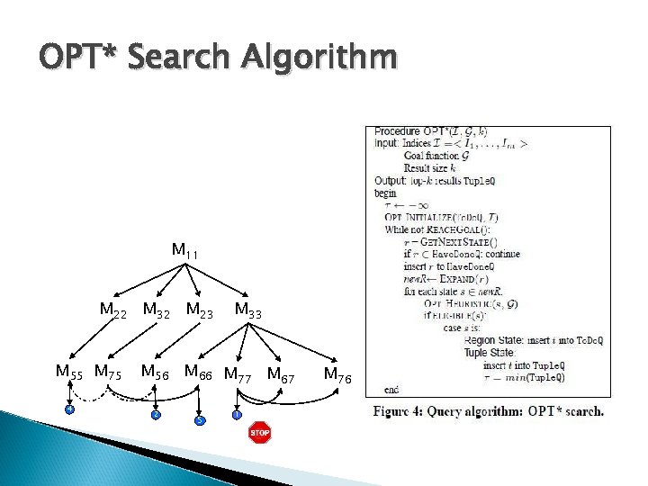
OPT* Search Algorithm M 11 M 22 M 32 M 23 M 55 M 75 4 M 33 M 56 M 66 M 77 M 67 2 5 1 M 76
Optimality of OPT* may result in different costs if started at different initial states. Top down-> More hops | Bottom up->Less hops Preference goes to Bottom Up but what if Goal functions G=1/(X-Y)2+1, any value satisfying X=Y maximizes the function.

Experiments Comparison vs. ◦ Boolean then ranking ◦ Ranking then boolean Metrics: node accessed = Nl + Nt Settings: ◦ Benchmark queries over real dataset ◦ Controlled queries over synthetic dataset 40

Benchmark queries Datasets: ◦ 19, 706 real estate listing crawled online Queries ◦ Q 1: size * bedrms/| price-450 k| : [40 k<=price<=50 k] ◦ Q 2: size * ebedrms / |price-350 k| : [price<400 k^size>4000] ◦ Q 3: size/price : [bedrms=3 ν bedrms=4] BR_clustered BR_unclustered OPT* Q 1 Q 2 Q 3 41

Controlled queries Datasets ◦ Three randomly generated datasets of 100 k points Uniform, gaussian, logvariatenormal Queries ◦ Linear average queries: (eg, 0. 4*a + 0. 6*b) ◦ Nearest neighbor queries: (eg, (x-3)^2 + (y-4)^2) ◦ Join queries: (0. 4*R. a + 0. 6*S. b: R. c=R. d) 42
Conclusion Problem ◦ Study K-constrained optimization queries as boolean + ranking Abstraction ◦ Encode K-constrained optimization into shortest path problem Framework ◦ Develop OPT* to process K-constrained optimization 43

• • References Boolean + Ranking: Querying a Database by K-Constrained Optimization. Z. Zhang, S. Hwang, K. C. -C. Chang, M. Wang, C. Lang, and Y. Chang. In Proceedings of the 2006 ACM SIGMOD Conference (SIGMOD 2006), pages 359 -370, Chicago, June 2006 www. wikipedia. org 44

Thank you! Questions? 45
b1aea55848b2e299e70f400bd5302de9.ppt