BMS 5525 Bioregulation Mon April 21 2008 A

BMS 5525 Bioregulation Mon. April 21, 2008 A Whirlwind Bioinformatics Survey. . . some taste of theory, and a few practicalities Steve Thompson Florida State University School of Computational Science (SCS)

To begin, some terminology — What is bioinformatics, genomics, proteomics, sequence analysis, computational molecular biology. . . ?

My definitions, lots of overlap Biocomputing and computational biology are synonyms and describe the use of computers and computational techniques to analyze any type of a biological system, from individual molecules to organisms to overall ecology. Bioinformatics describes using computational techniques to access, analyze, and interpret the biological information in any type of biological database. Sequence analysis is the study of molecular sequence data for the purpose of inferring the function, interactions, evolution, and perhaps structure of biological molecules. Genomics analyzes the context of genes or complete genomes (the total DNA content of an organism) within the same and/or across different genomes. Proteomics is the subdivision of genomics concerned with analyzing the complete protein complement, i. e. the proteome, of organisms, both within and between different organisms.

And one way to think about it — the Reverse Biochemistry Analogy Biochemists no longer have to begin a research project by isolating and purifying massive amounts of a protein from its native organism in order to characterize a particular gene product. Rather, now scientists can amplify a section of some genome based on its similarity to other genomes, sequence that piece of DNA and, using sequence analysis tools, infer all sorts of functional, regulatory, evolutionary, and, perhaps, structural insight into that stretch of DNA! The computer and molecular databases are a necessary, integral part of this entire process.

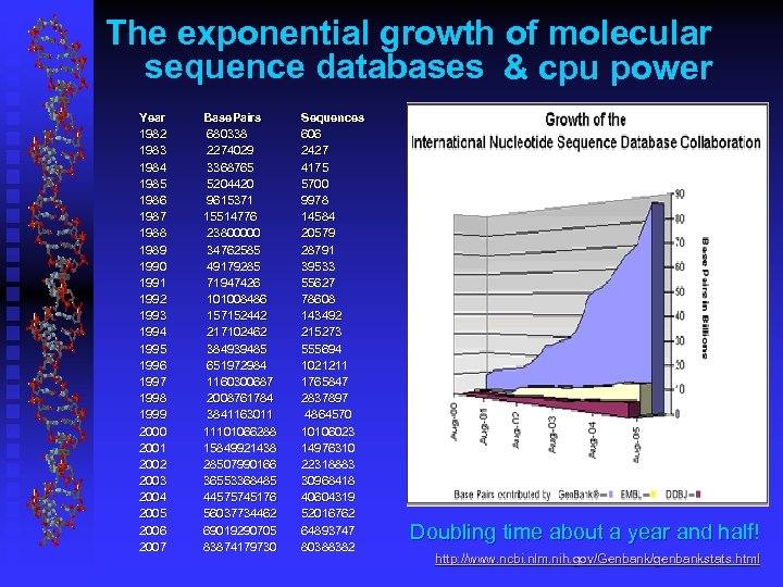
The exponential growth of molecular sequence databases & cpu power Year 1982 1983 1984 1985 1986 1987 1988 1989 1990 1991 1992 1993 1994 1995 1996 1997 1998 1999 2000 2001 2002 2003 2004 2005 2006 2007 Base. Pairs 680338 2274029 3368765 5204420 9615371 15514776 23800000 34762585 49179285 71947426 101008486 157152442 217102462 384939485 651972984 1160300687 2008761784 3841163011 11101066288 15849921438 28507990166 36553368485 44575745176 56037734462 69019290705 83874179730 Sequences 606 2427 4175 5700 9978 14584 20579 28791 39533 55627 78608 143492 215273 555694 1021211 1765847 2837897 4864570 10106023 14976310 22318883 30968418 40604319 52016762 64893747 80388382 Doubling time about a year and half! http: //www. ncbi. nlm. nih. gov/Genbank/genbankstats. html

Sequence database growth, continued The International Human Genome Sequencing Consortium announced the completion of the "Working Draft" of the human genome in June 2000; independently that same month, the private company Celera Genomics announced that it had completed the first “Assembly” of the human genome. The classic articles were published mid-February 2001 in the journals Science and Nature. Genome projects keep the data coming at an incredible rate. Currently around 50 Archaea, 600 Bacteria, and 20 Eukaryote complete genomes, and 200 Eukaryote assemblies are represented, not counting the almost 3, 000 virus and viroid genomes available.

Some neat stuff from the human genome papers Homo sapiens, aren’t nearly as special as we once thought. Of the 3. 2 billion base pairs in our DNA: Traditional gene number estimates were often in the 100, 000 range; turns out we’ve only got about twice as many as a fruit fly, between 25’ and 30, 000! The protein coding region of the genome is only about 1% or so, a bunch of the remainder is ‘jumping, ’ ‘selfish DNA, ’ sometimes called ‘junk, ’ much of which may be involved in regulation and control. Some 100 -200 genes were transferred from an ancestral bacterial genome to an ancestral vertebrate genome! (Later shown to be false by more extensive analyses, and to be due to gene loss not transfer. )

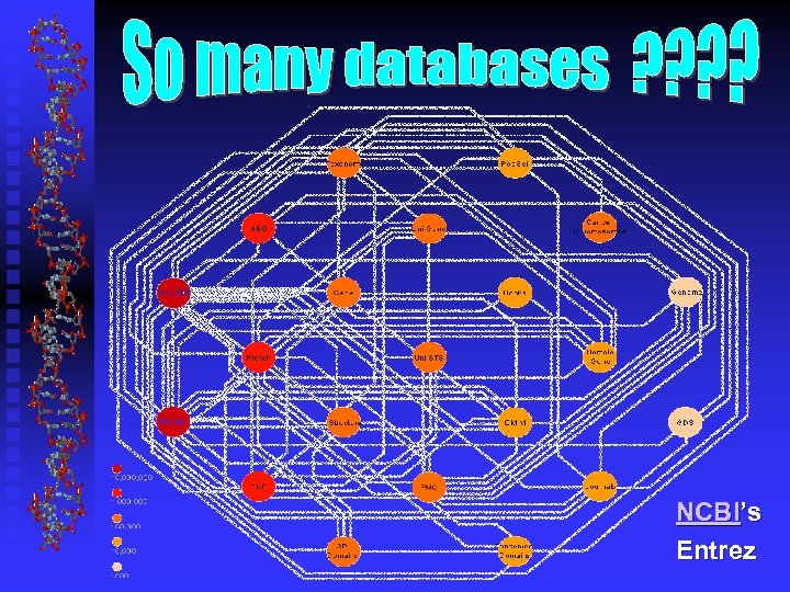
NCBI’s Entrez

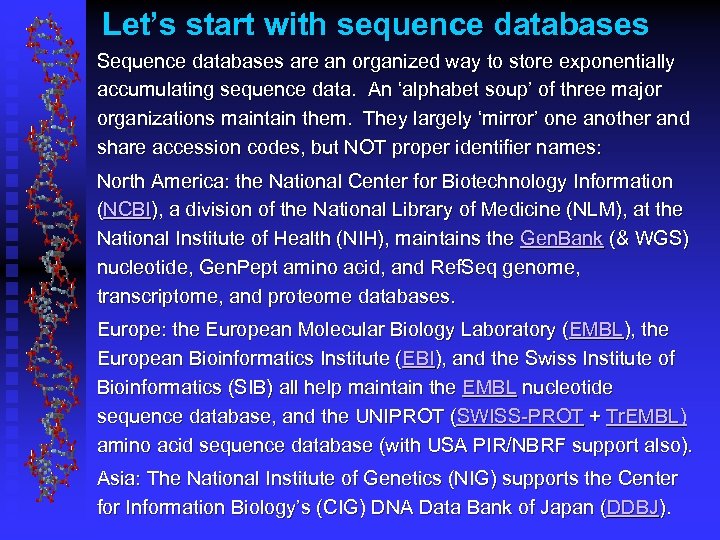
Let’s start with sequence databases Sequence databases are an organized way to store exponentially accumulating sequence data. An ‘alphabet soup’ of three major organizations maintain them. They largely ‘mirror’ one another and share accession codes, but NOT proper identifier names: North America: the National Center for Biotechnology Information (NCBI), a division of the National Library of Medicine (NLM), at the National Institute of Health (NIH), maintains the Gen. Bank (& WGS) nucleotide, Gen. Pept amino acid, and Ref. Seq genome, transcriptome, and proteome databases. Europe: the European Molecular Biology Laboratory (EMBL), the European Bioinformatics Institute (EBI), and the Swiss Institute of Bioinformatics (SIB) all help maintain the EMBL nucleotide sequence database, and the UNIPROT (SWISS-PROT + Tr. EMBL) amino acid sequence database (with USA PIR/NBRF support also). Asia: The National Institute of Genetics (NIG) supports the Center for Information Biology’s (CIG) DNA Data Bank of Japan (DDBJ).

A little history The first well recognized sequence database was Dr. Margaret Dayhoff’s hardbound Atlas of Protein Sequence and Structure begun in the mid-sixties. That became PIR. DDBJ began in 1984, Gen. Bank in 1982, and EMBL in 1980. They are all attempts at establishing an organized, reliable, comprehensive, and openly available library of genetic sequences. Sequence databases have long-since outgrown a hardbound atlas that you can pull off of a library shelf. They have become gargantuan and have evolved through many, many changes.

What are sequence databases like? Just what are primary sequences? (Central Dogma: DNA —> RNA —> protein) Primary refers to one dimension — all of the ‘symbol’ information written in sequential order necessary to specify a particular biological molecular entity, be it polypeptide or nucleotide. The symbols are the one letter codes for all of the biological nitrogenous bases and amino acid residues and their ambiguity codes. Biological carbohydrates, lipids, and structural and functional information are not sequence data. Not even DNA CDS protein translations in a DNA database are sequence data! However, much of this feature and bibliographic type information is available in the reference documentation sections associated with primary sequences in the databases. Software is required to successfully interact with these databases, and access is most easily handled through various software packages and interfaces, on the World Wide Web or otherwise.

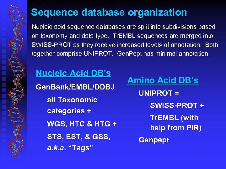
Sequence database organization Nucleic acid sequence databases are split into subdivisions based on taxonomy and data type. Tr. EMBL sequences are merged into SWISS-PROT as they receive increased levels of annotation. Both together comprise UNIPROT. Gen. Pept has minimal annotation. Nucleic Acid DB’s Gen. Bank/EMBL/DDBJ all Taxonomic categories + WGS, HTC & HTG + STS, EST, & GSS, a. k. a. “Tags” Amino Acid DB’s UNIPROT = SWISS-PROT + Tr. EMBL (with help from PIR) Genpept

Parts and problems Important elements associated with each sequence entry: Name: LOCUS, ENTRY, ID, all are unique identifiers. Definition: a. k. a. title, a brief textual sequence description. Accession Number: a constant data identifier. Source and taxonomy information; complete literature references; comments and keywords; and the all important FEATURE table! A summary or checksum line, and the sequence itself. However: Each major database as well as each major suite of software tools has its own distinct format requirements. Changes over the years are a huge hassle. Standards are argued, e. g. XML, but unfortunately, until all biologists and computer scientists worldwide agree on one standard, and all software is (re)written to that standard, neither of which is likely to happen very quickly, if ever, format issues will remain one of the most confusing and troubling aspects of working with sequence data. Specialized format conversion tools expedite the chore, but becoming familiar with some of the common formats helps a lot.

More format complications Indels and missing data symbols (i. e. gaps) designation discrepancy headaches — . , -, ~, ? , N, or X. . . Help!

Specialized ‘sequence’ -type databases Databases that contain special types of sequence information, such as patterns, motifs, and profiles. These include: REBASE, EPD, PROSITE, BLOCKS, Pro. Dom, Pfam. . Databases that contain multiple sequence entries aligned, e. g. Pop. Set, RDP and ALN. Databases that contain families of sequences ordered functionally, structurally, or phylogenetically, e. g. i. Pro. Class and HOVERGEN. Databases of species specific sequences, e. g. the HIV Database and the Giardia lamblia Genome Project. And on and on. . See Amos Bairoch’s excellent links page: http: //us. expasy. org/alinks. html.

What about other types of biological databases? Three-dimensional structure databases The Protein Data Bank and Rutgers Nucleic Acid Database. See Molecules to Go at http: //molbio. info. nih. gov/cgi-bin/pdb/. These databases contain all of the 3 D atomic coordinate data necessary to define the tertiary shape of a particular biological molecule. The data is usually experimentally derived, either by Xray crystallography or by NMR, sometimes it’s hypothetical. Secondary structure boundaries, sequence data, source, resolution, and references are given in the annotation. These databases enable the technique of homology modeling to actually work pretty well given your sequence is similar enough to solved structures (see the automated Swiss-Model server at http: //swissmodel. expasy. org/SWISS-MODEL. html). Molecular visualization and/or modeling software is required to interact with the data. It has little meaning on its own.

And still other types of bioinfo’ databases Consider these ‘non-molecular’ but they often link to molecules: Reference Databases (all w/ pointers to sequences): e. g. Locus. Link/Gene — integrated knowledge base OMIM — Online Mendelian Inheritance in Man Pub. Med/Med. Line — over 11 million citations from more than 4 thousand bio/medical scientific journals. Phylogenetic Tree Databases: e. g. the Tree of Life. Metabolic Pathway Databases: e. g. WIT (What Is There), Japan’s Genome. Net KEGG (the Kyoto Encyclopedia of Genes and Genomes), and the human Reactome. Population studies data — which strains, where, etc. And then databases that many biocomputing people don’t even usually consider: e. g. GIS/GPS/remote sensing data, medical records, census counts, mortality and birth rates. .

OK, but what can you do with new genomic sequence data without annotation? Easy — restriction digests and associated mapping. Harder — fragment and genome assembly; such as packages from the University of Washington’s Genome Center (http: //www. genome. washington. edu/), Phred/Phrap/Consed (http: //www. phrap. org/), and The Institute for Genomic Research’s (http: //www. tigr. org/) Lucy and Assembler programs. Very hard — gene finding and sequence annotation. What’s it all mean! This is a primary focus of genomics research, and we’ll use it as a theme today. Easy— forward translation to peptides after genes (and all intron/exon strructure) are identified. Hard again — genome scale comparisons and analyses. The BIG picture — structure, function, regulation, evolution.

Therefore, genome characterization: Recognizing coding sequences Three general solutions to the gene finding problem: 1) all genes have particular regulatory signals near them, 2) all genes by definition contain specific code patterns, 3) and many genes have already been characterized in other organisms so we can infer function and location by homology if our new sequence is similar enough to an existing sequence. All of these principles can be used to help locate the position of genes in DNA, and are often known as “searching by signal, ” “searching by content, ” and “homology inference” respectively. We’ll illustrate these concepts in the rest of today’s lecture — and, hopefully, you’ll learn about much of bioinformatics in the process!

So, given some biological sequence data, what more can we learn about its evolution, structure, function, mechanism and regulation in life? Enter pairwise alignment, similarity searching, significance, and homology.

First, just what is homology and similarity — are they the same? Don’t confuse homology with similarity: there is a huge difference! Similarity is a statistic that describes how much two (sub)sequences are alike according to some set scoring criteria. It can be normalized to ascertain statistical significance, but it’s still just a number.

Homology, in contrast and by definition implies an evolutionary relationship — more than just everything evolving from the same primordial ‘ooze. ’ Reconstruct the phylogeny of the organisms or genes of interest to demonstrate homology. Better yet, show experimental evidence — structural, morphological, genetic, and/or fossil — that corroborates your claim. There is no such thing as percent homology; something is either homologous or it is not. Walter Fitch said “homology is like pregnancy — you can’t be 45% pregnant, just like something can’t be 45% homologous. You either are or you are not. ” Highly significant similarity can argue for homology, but not the inverse.

OK, so how can we see if two sequences are similar? First, to introduce the concept, a graphical method. . . One way — dot matrices. Provide a ‘Gestalt’ of all possible alignments between two sequences. To begin — very simple 0, 1 (match, nomatch) identity scoring function. Put a dot wherever symbols match.

Identities and insertion/deletion events (indels) identified (zero: one match score matrix, no window).

Noise due to random composition effects contributes to confusion. To ‘clean up’ the plot consider a filtered windowing approach. A dot is placed at the middle of a window if some ‘stringency’ is met within that defined window size. Then the window is shifted one position and the entire process is repeated (zero: one match score, window of size three and a stringency level of two out of three).

Exact alignment — but how can we ‘see’ the correspondence of individual residues? We can compare one molecule against another by aligning them. However, a ‘brute force’ approach just won’t work. Even without considering the introduction of gaps, the computation required to compare all possible alignments between two sequences requires time proportional to the product of the lengths of the two sequences. Therefore, if the two sequences are approximately the same length (N), this is a N 2 problem. To include gaps, we would have to repeat the calculation 2 N times to examine the possibility of gaps at each possible position within the sequences, now a N 4 N problem. There’s no way! We need an algorithm.

But. . . Just what the heck is an algorithm? Merriam-Webster’s says: “A rule of procedure for solving a problem [often mathematical] that frequently involves repetition of an operation. ” So, you could write an algorithm for tying your shoe! It’s just a set of explicit instructions for doing some routine task.

Enter the Dynamic Programming Algorithm! Computer scientists figured it out long ago; Needleman and Wunsch applied it to the alignment of the full lengths of two sequences in 1970. An optimal alignment is defined as an arrangement of two sequences, 1 of length i and 2 of length j, such that: 1) 2) 3) you maximize the number of matching symbols between 1 and 2; you minimize the number of indels within 1 and 2; and you minimize the number of mismatched symbols between 1 and 2. Therefore, the actual solution can be represented by: Si-1 j-1 or max Si-x j-1 + wx-1 or Sij = sij + max 2 < x < i max Si-1 j-y + wy-1 2<y<I Where Sij is the score for the alignment ending at i in sequence 1 and j in sequence 2, sij is the score for aligning i with j, wx is the score for making a x long gap in sequence 1, wy is the score for making a y long gap in sequence 2, allowing gaps to be any length in either sequence.

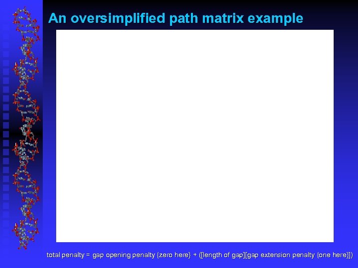
An oversimplified path matrix example total penalty = gap opening penalty {zero here} + ([length of gap][gap extension penalty {one here}])

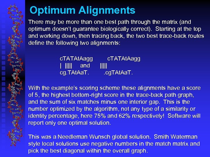
Optimum Alignments There may be more than one best path through the matrix (and optimum doesn’t guarantee biologically correct). Starting at the top and working down, then tracing back, the two best trace-back routes define the following two alignments: c. TATAt. Aagg | ||||| and cg. TAt. Aa. T. c. TATAt. Aagg |||||. cg. TAt. Aa. T. With the example’s scoring scheme these alignments have a score of 5, the highest bottom-right score in the trace-back path graph, and the sum of six matches minus one interior gap. This is the number optimized by the algorithm, not any type of a similarity or identity percentage, here 75% and 62% respectively! Software will report only one optimal solution. This was a Needleman Wunsch global solution. Smith Waterman style local solutions use negative numbers in the match matrix and pick the best diagonal within the overall graph.

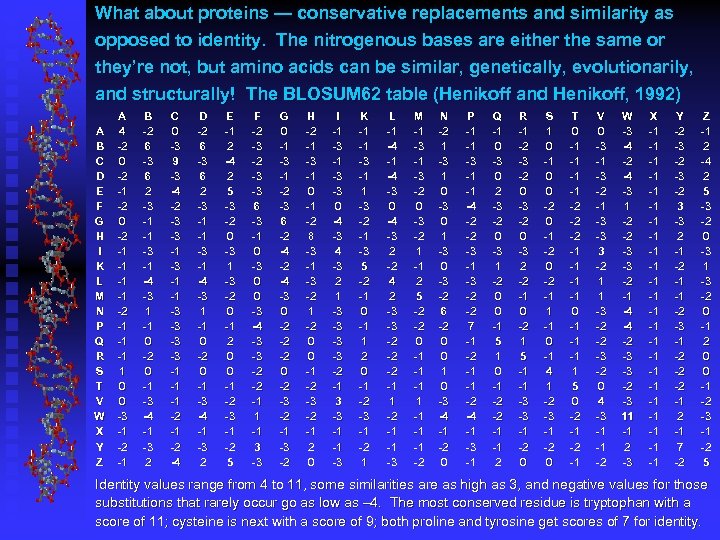
What about proteins — conservative replacements and similarity as opposed to identity. The nitrogenous bases are either the same or they’re not, but amino acids can be similar, genetically, evolutionarily, and structurally! The BLOSUM 62 table (Henikoff and Henikoff, 1992) A B C D E F G H I K L M N P Q R S T V W X Y Z A 4 -2 0 -2 -1 -1 -2 -1 -1 -1 1 0 0 -3 -1 -2 -1 B -2 6 -3 6 2 -3 -1 -1 -3 -1 -4 -3 1 -1 0 -2 0 -1 -3 -4 -1 -3 2 C 0 -3 9 -3 -4 -2 -3 -3 -1 -1 -1 -2 -4 D -2 6 -3 6 2 -3 -1 -1 -3 -1 -4 -3 1 -1 0 -2 0 -1 -3 -4 -1 -3 2 E -1 2 -4 2 5 -3 -2 0 -3 1 -3 -2 0 -1 2 0 0 -1 -2 -3 -1 -2 5 F -2 -3 -3 6 -3 -1 0 -3 0 0 -3 -4 -3 -3 -2 -2 -1 1 -1 3 -3 G 0 -1 -3 -1 -2 -3 6 -2 -4 -3 0 -2 -2 -2 0 -2 -3 -2 -1 -3 -2 H -2 -1 -3 -1 0 -1 -2 8 -3 -1 -3 -2 1 -2 0 0 -1 -2 -3 -2 -1 2 0 I -1 -3 -3 0 -4 -3 2 1 -3 -3 -2 -1 3 -3 -1 -1 -3 K -1 -1 -3 -1 1 -3 -2 -1 -3 5 -2 -1 0 -1 1 2 0 -1 -2 -3 -1 -2 1 L -1 -4 -3 0 -4 -3 2 -2 4 2 -3 -3 -2 -2 -2 -1 1 -2 -1 -1 -3 M -1 -3 -2 0 -3 -2 1 -1 2 5 -2 -2 0 -1 -1 -2 N -2 1 -3 1 0 -3 0 1 -3 0 -3 -2 6 -2 0 0 1 0 -3 -4 -1 -2 0 P -1 -1 -3 -1 -1 -4 -2 -2 -3 -1 -3 -2 -2 7 -1 -2 -1 -1 -2 -4 -1 -3 -1 Q -1 0 -3 0 2 -3 -2 0 -3 1 -2 0 0 -1 5 1 0 -1 -2 -2 -1 -1 2 R -1 -2 -3 -2 0 -3 2 -2 -1 0 -2 1 5 -1 -1 -3 -3 -1 -2 0 S 1 0 -1 0 0 -2 0 -1 -2 0 -2 -1 1 -1 0 -1 4 1 -2 -3 -1 -2 0 T 0 -1 -1 -2 -2 -2 -1 -1 0 -1 -1 -1 1 5 0 -2 -1 V 0 -3 -1 -3 -2 -1 -3 -3 3 -2 1 1 -3 -2 -2 -3 -2 0 4 -3 -1 -1 -2 W -3 -4 -2 -4 -3 1 -2 -2 -3 -3 -2 -1 -4 -4 -2 -3 -3 -2 -3 11 -1 2 -3 X -1 -1 -1 -1 -1 -1 Y -2 -3 -2 3 -3 2 -1 -1 -2 -3 -1 -2 -2 -2 -1 7 -2 Z -1 2 -4 2 5 -3 -2 0 -3 1 -3 -2 0 -1 2 0 0 -1 -2 -3 -1 -2 5 Identity values range from 4 to 11, some similarities are as high as 3, and negative values for those substitutions that rarely occur go as low as – 4. The most conserved residue is tryptophan with a score of 11; cysteine is next with a score of 9; both proline and tyrosine get scores of 7 for identity.

We can imagine screening databases for sequences similar to ours using these concepts of dynamic programming and substitution scoring matrices and some yet to be described algorithmic tricks. But what do database searches tell us; what can we gain from them? Why even bother? Inference through homology is a fundamental principle of When a sequence is found to fall into a preexisting family biology!be able recognize genes, and infer function, we may regulation, mechanism, evolution, and perhaps even structure, based on homology with its neighbors.

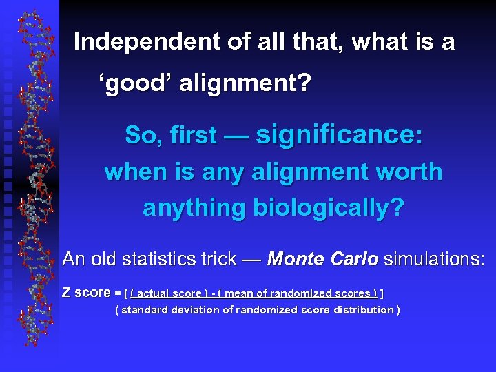
Independent of all that, what is a ‘good’ alignment? So, first — significance: when is any alignment worth anything biologically? An old statistics trick — Monte Carlo simulations: Z score = [ ( actual score ) - ( mean of randomized scores ) ] ( standard deviation of randomized score distribution )

The Normal distribution Many Z scores measure the distance from the mean using this simplistic Monte Carlo model assuming a Gaussian distribution, a. k. a. the Normal distribution (http: //mathworld. wolfram. com/Normal. Distribution. html), in spite of the fact that ‘sequence-space’ actually follows what is know as the ‘Extreme Value distribution. ’ However, the Monte Carlo method does approximate significance estimates fairly well.

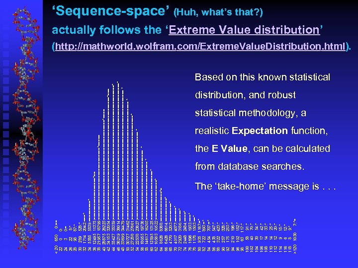
< 20 650 0: == 22 0 0: 24 3 0: = 26 22 8: * 28 98 87: * 30 289 528: * 32 1714 2042: ===* 34 5585 5539: =====* 36 12495 11375: =========*== 38 21957 18799: ================*===== 40 28875 26223: ======================*==== 42 34153 32054: ===========================*=== 44 35427 35359: =============================* 46 36219 36014: ==============================* 48 33699 34479: ============================ * 50 30727 31462: ========================== * 52 27288 27661: =======================* 54 22538 23627: =================== * 56 18055 19736: =============== * 58 14617 16203: ============= * 60 12595 13125: ===========* 62 10563 10522: =========* 64 8626 8368: =======*= 66 6426 6614: =====* 68 4770 5203: ====* 70 4017 4077: ======* 72 2920 3186: =====* 74 2448 2484: ====* 76 1696 1933: ===* 78 1178 1503: ==* 80 935 1167: =* 82 722 893: =* 84 454 707: =* 86 438 547: * 88 322 423: * 90 257 328: * 92 175 253: * 94 210 196: * 96 102 152: * 98 63 117: * 100 58 91: * 102 40 70: * 104 30 54: * 106 17 42: * 108 14 33: * 110 14 25: * 112 12 20: * 114 9 15: * 116 6 12: * 118 8 9: * >120 1030 7: *= ‘Sequence-space’ (Huh, what’s that? ) actually follows the ‘Extreme Value distribution’ (http: //mathworld. wolfram. com/Extreme. Value. Distribution. html). Based on this known statistical distribution, and robust statistical methodology, a realistic Expectation function, the E Value, can be calculated from database searches. The ‘take-home’ message is. . .

The Expectation Value! The higher the E value is, the more probable that the observed match is due to chance in a search of the same size database, and the lower its Z score will be, i. e. is NOT significant. Therefore, the smaller the E value, i. e. the closer it is to zero, the more significant it is and the higher its Z score will be! The E value is the number that really matters. In other words, in order to assess whether a given alignment constitutes evidence for homology, it helps to know how strong an alignment can be expected from chance alone.

Rules of thumb for a protein search The Z score represents the number of standard deviations some particular alignment is from a distribution of random alignments (often the Normal distribution). They very roughly correspond to the listed E Values (based on the Extreme Value distribution) for a typical protein sequence similarity search through a database with ~250, 000 protein entries.

On to the searches How can you search the databases for similar sequences, if pairwise alignments take N 2 time? ! Significance and heuristics. . . Database searching programs use the two concepts of dynamic programming and substitution scoring matrices; however, dynamic programming takes far too long when used against most sequence databases with a ‘normal’ computer. Remember how big the databases are! Therefore, the programs use tricks to make things happen faster. These tricks fall into two main categories, that of hashing, and that of approximation.

Corn beef hash? Huh. . . Hashing is the process of breaking your sequence into small ‘words’ or ‘k-tuples’ (think all chopped up, just like corn beef hash) of a set size and creating a ‘look-up’ table with those words keyed to position numbers. Computers can deal with numbers way faster than they can deal with strings of letters, and this preprocessing step happens very quickly. Then when any of the word positions match part of an entry in the database, that match, the ‘offset, ’ is saved. In general, hashing reduces the complexity of the search problem from N 2 for dynamic programming to N, the length of all the sequences in the database.

OK. Heuristics. . . What’s that? Approximation techniques are collectively known as ‘heuristics. ’ Webster’s defines heuristic as “serving to guide, discover, or reveal; . . . but unproved or incapable of proof. ” In database similarity searching techniques the heuristic usually restricts the necessary search space by calculating some sort of a statistic that allows the program to decide whether further scrutiny of a particular match should be pursued. This statistic may miss things depending on the parameters set — that’s what makes it heuristic. ‘Worthwhile’ results at the end are compiled and the longest alignment within the program’s restrictions is created. The exact implementation varies between the different programs, but the basic idea follows in most all of them.

Two predominant versions exist: BLAST and Fast Both return local alignments, and are not a single program, but rather a family of programs with implementations designed to compare a sequence to a database every which way. These include: 1) a DNA sequence against a DNA database (not recommended unless forced to do so because you are dealing with a non-translated region of the genome — DNA is just too darn noisy, only identity & four bases!), 2) a translated (where the translation is done ‘on-the-fly’ in all six frames) version of a DNA sequence against a translated (‘on-the-fly’ six-frame) version of the DNA database (not available in the Fast package), 3) a translated (‘on-the-fly’ six-frame) version of a DNA sequence against a protein database, 4) a protein sequence against a translated (‘on-the-fly’ six-frame) version of a DNA database, 5) or a protein sequence against a protein database. Translated comparisons allow penalty-free frame shifts.

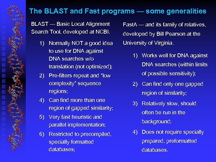
The BLAST and Fast programs — some generalities BLAST — Basic Local Alignment Search Tool, developed at NCBI. 1) Normally NOT a good idea to use for DNA against DNA searches w/o translation (not optimized); Fast. A — and its family of relatives, developed by Bill Pearson at the University of Virginia. 1) Works well for DNA against DNA searches (within limits of possible sensitivity); 2) Pre-filters repeat and “low complexity” sequence regions; 2) Can find only one gapped 4) Can find more than one region of gapped similarity; 3) Relatively slow, should 5) Very fast heuristic and parallel implementation; 6) Restricted to precompiled, specially formatted databases; region of similarity; often be run in the background; 4) Does not require specially prepared, preformatted databases.

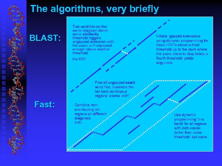
The algorithms, very briefly BLAST: Two word hits on the same diagonal above some similarity threshold triggers ungapped extension until the score isn’t improved enough above another threshold: the HSP. Initiate gapped extensions using dynamic programming for those HSP’s above a third threshold up to the point where the score starts to drop below a fourth threshold: yields alignment. Find all ungapped exact word hits; maximize the ten best continuous regions’ scores: init 1. Fast: Combine nonoverlapping init regions on different diagonals: initn. Use dynamic programming ‘in a band’ for all regions with initn scores better than some threshold: opt score.

What’s the deal with DNA versus protein for searches and alignment? All database similarity searching and sequence alignment, regardless of the algorithm used, is far more sensitive at the amino acid level than at the DNA level. This is because proteins have twenty match criteria versus DNA’s four, and those four DNA bases can generally only be identical, not similar, to each other; and many DNA base changes (especially third position changes) do not change the encoded protein. All of these factors drastically increase the ‘noise’ level of a DNA against DNA search, and give protein searches a much greater ‘look-back’ time, at least doubling it. Therefore, whenever dealing with coding sequence, it is always prudent to search at the protein level!

What can we do with the significant results of database searching — multiple sequence alignment & analysis — why even bother? More data yields stronger analyses — as long as it is done carefully! Mosaic ideas and evolutionary ‘importance. ’ Applications: Probe, primer, and motif design; Graphical illustrations; Comparative ‘homology’ inference; Molecular evolutionary analysis. All right — how do you do it?

Dynamic programming’s complexity increases exponentially with the number of sequences being compared: N-dimensional matrix. . complexity=[sequence length]number of sequences i. e. complexity is O(en)

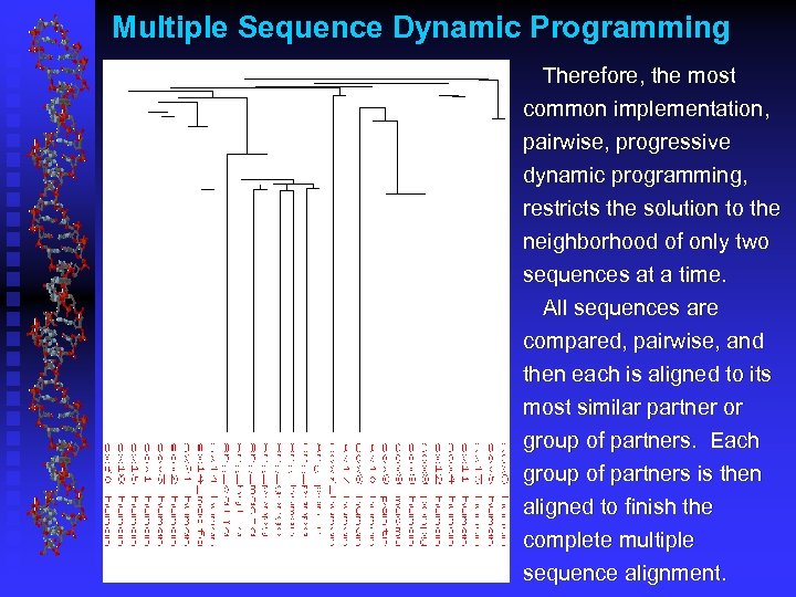
Multiple Sequence Dynamic Programming Therefore, the most common implementation, pairwise, progressive dynamic programming, restricts the solution to the neighborhood of only two sequences at a time. All sequences are compared, pairwise, and then each is aligned to its most similar partner or group of partners. Each group of partners is then aligned to finish the complete multiple sequence alignment.

Web resources for pairwise, progressive multiple alignment in the USA, include the Baylor College of Medicine’s Search Launcher — http: //searchlauncher. bcm. tmc. edu/ However, problems with large datasets and huge multiple alignments make doing multiple sequence alignment on the Web impractical after your dataset has reached a certain size. You’ll know it when you’re there!

So, what else is available? Stand-alone Clustal. W is available for all operating systems; its graphical user interface Clustal. X, makes running it very easy. And dedicated biocomputing server suites, like the GCG Wisconsin Package, which includes Pile. Up and Clustal. W and the Seq. Lab graphical user interface, are another powerful solution. Furthermore, newer software such as TCoffee, MUSCLE, Prob. Cons, POA, MAFFT, etc. add various tweaks and tricks to make the entire process more accurate and/or faster.

Reliability and the Comparative Approach explicit homologous correspondence; manual adjustments based on knowledge, especially structural, regulatory, and functional sites. Therefore, editors like Seq. Lab and structure based databses like the Ribosomal Database Project: http: //rdp. cme. msu. edu/index. jsp

Structural & Functional correspondence in the Wisconsin Package’s Seq. Lab

As with pairwise methods, work with proteins! If at all possible Twenty match symbols versus four, plus similarity! Way better signal to noise. Also guarantees no indels are placed within codons. So translate, then align. Nucleotide sequences will only reliably align if they are very similar to each other. And they will require extensive hand editing and careful consideration.

Beware of aligning apples and oranges [and grapefruit]! Receptor versus activator, on ad nauseam; parologue versus orthologue; genomic versus c. DNA; mature versus precursor.

Mask out uncertain areas

Complications — Order dependence. Not that big of a deal. Substitution matrices and gap penalties. A very big deal! Regional ‘realignment’ becomes incredibly important, especially with sequences that have areas of high and low similarity

Homology inference is especially powerful for finding genes and functional and regulatory domains within them! The information within a multiple sequence alignment can dramatically point to evolutionarily constrained elements in the sequences. Furthermore, often functions can experimentally be ascribed to them. Therefore, we can search for those elements in unknown sequences to attempt to identify the unknown’s function. How does this work?

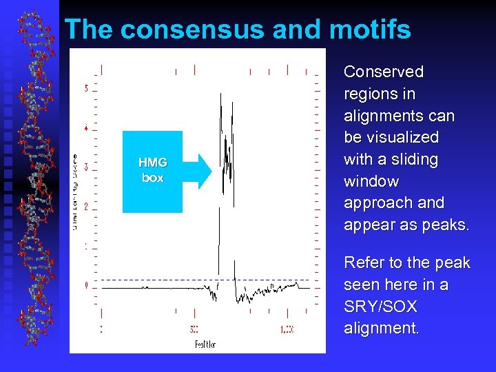
The consensus and motifs HMG box Conserved regions in alignments can be visualized with a sliding window approach and appear as peaks. Refer to the peak seen here in a SRY/SOX alignment.

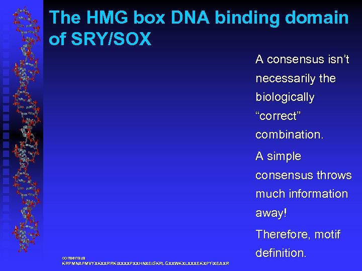
The HMG box DNA binding domain of SRY/SOX A consensus isn’t necessarily the biologically “correct” combination. A simple consensus throws much information away! Therefore, motif consensus KRPMNAFMVYXKXXRRKIXXXXPXXHNXEISKRLGXXWKXLXXXEKXPYIXEAXR definition.

PROSITE, a simple fast approach The trick is to define a motif such that it minimizes false positives and maximizes true positives — it needs to be just discriminatory enough. Development is largely empirical; a pattern is made, tested against the database, then refined, over and over, although when experimental evidence is available, it is always incorporated. This is known as motif definition and Amos Bairoch, has done it a bunch! His database of catalogued structural, regulatory, and enzymatic consensus patterns or ‘signatures’ is the PROSITE Database of protein families and domains and contains 1, 510 documentation entries that describe 2, 877 different patterns, rules, and profiles/matrices (Release 20. 77, Feb. 26, 2008). Pattern descriptions for these characteristic local sequence areas are variously and confusingly known as motifs, templates, signatures, patterns, and even fingerprints.

The HMG box — Defined as: [FI]-S-[KR]-K-C-x[EK]-R-W-K-T-M. A one-dimensional ‘regular-expression’ of a conserved site. Not necessarily biologically meaningful though, and motifs are limited in their ability to discriminate a residue’s ‘importance. ’

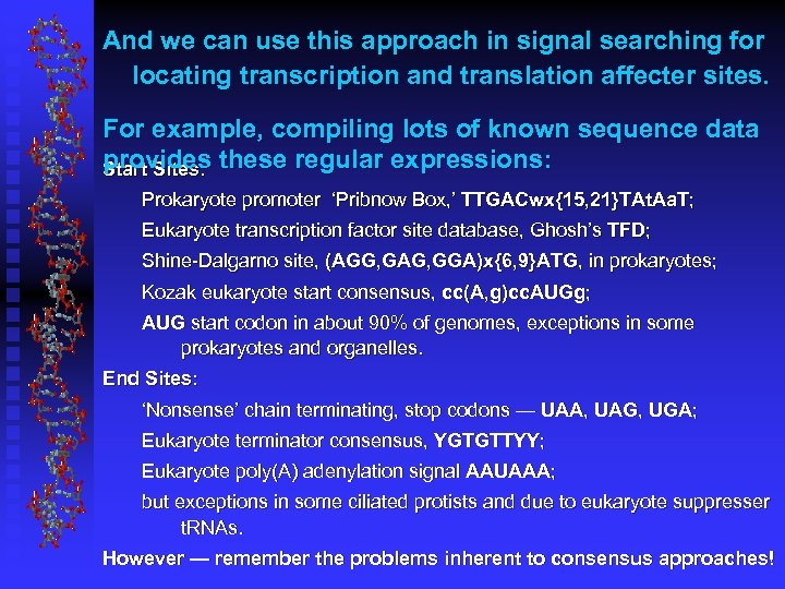
And we can use this approach in signal searching for locating transcription and translation affecter sites. For example, compiling lots of known sequence data provides these regular expressions: Start Sites: Prokaryote promoter ‘Pribnow Box, ’ TTGACwx{15, 21}TAt. Aa. T; Eukaryote transcription factor site database, Ghosh’s TFD; Shine-Dalgarno site, (AGG, GAG, GGA)x{6, 9}ATG, in prokaryotes; Kozak eukaryote start consensus, cc(A, g)cc. AUGg; AUG start codon in about 90% of genomes, exceptions in some prokaryotes and organelles. End Sites: ‘Nonsense’ chain terminating, stop codons — UAA, UAG, UGA; Eukaryote terminator consensus, YGTGTTYY; Eukaryote poly(A) adenylation signal AAUAAA; but exceptions in some ciliated protists and due to eukaryote suppresser t. RNAs. However — remember the problems inherent to consensus approaches!

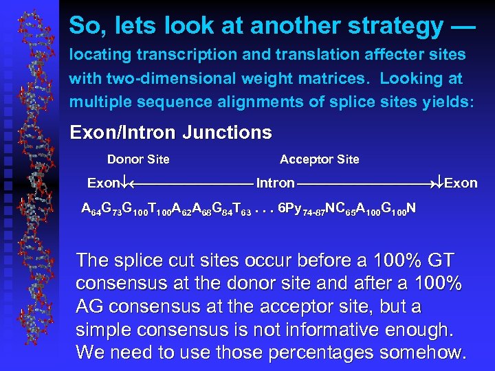
So, lets look at another strategy — locating transcription and translation affecter sites with two-dimensional weight matrices. Looking at multiple sequence alignments of splice sites yields: Exon/Intron Junctions Donor Site Acceptor Site Exon Intron Exon A 64 G 73 G 100 T 100 A 62 A 68 G 84 T 63. . . 6 Py 74 -87 NC 65 A 100 G 100 N The splice cut sites occur before a 100% GT consensus at the donor site and after a 100% AG consensus at the acceptor site, but a simple consensus is not informative enough. We need to use those percentages somehow.

To do that we need to include ‘all’ of the information from the multiple sequence alignment, or of some region within the alignment, in a description that doesn’t throw anything away! Enter — two-dimensional techniques for homology searching — the PSSM (position specific site matrix) and the ‘profile’ algorithms, including Psi. BLAST, MEME, and HMMer. . . How do these work?

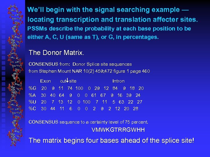
We’ll begin with the signal searching example — locating transcription and translation affecter sites. PSSMs describe the probability at each base position to be either A, C, U (same as T), or G, in percentages. The Donor Matrix. CONSENSUS from: Donor Splice site sequences from Stephen Mount NAR 10(2) 459; 472 figure 1 page 460 Exon %G 20 9 %A 30 40 %U 20 7 %C 30 44 cut site Intron 11 74 100 0 29 12 84 9 18 20 64 9 0 0 61 67 9 16 39 24 13 12 0 100 7 11 5 63 22 27 11 6 0 0 2 9 2 12 20 28 CONSENSUS sequence to a certainty level of 75 percent. VMWKGTRRGWHH The matrix begins four bases ahead of the splice site!

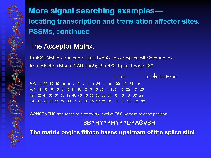
More signal searching examples— locating transcription and translation affecter sites. PSSMs, continued The Acceptor Matrix. CONSENSUS of: Acceptor. Dat. IVS Acceptor Splice Site Sequences from Stephen Mount NAR 10(2); 459 -472 figure 1 page 460 cut site Exon Intron %G 15 22 10 10 10 6 7 9 7 5 5 24 1 0 100 52 24 19 %A 15 10 10 15 6 15 11 19 12 3 10 25 4 100 0 22 17 20 %T 52 44 50 54 60 49 48 45 45 57 58 30 31 0 0 %C 18 25 30 21 24 30 34 28 36 35 27 21 64 0 0 18 22 32 8 37 29 CONSENSUS sequence to a certainty level of 75. 0 percent at each position: BBYHYYYDYAGVBH The matrix begins fifteen bases upstream of the splice site!

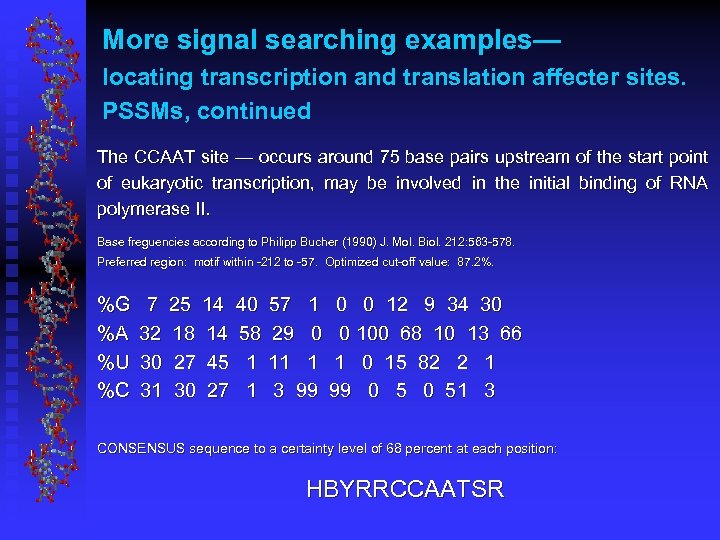
More signal searching examples— locating transcription and translation affecter sites. PSSMs, continued The CCAAT site — occurs around 75 base pairs upstream of the start point of eukaryotic transcription, may be involved in the initial binding of RNA polymerase II. Base freguencies according to Philipp Bucher (1990) J. Mol. Biol. 212: 563 -578. Biol. Preferred region: motif within -212 to -57. Optimized cut-off value: 87. 2%. %G %A %U %C 7 25 14 40 57 1 0 0 12 9 34 30 32 18 14 58 29 0 0 100 68 10 13 66 30 27 45 1 11 1 1 0 15 82 2 1 31 30 27 1 3 99 99 0 51 3 CONSENSUS sequence to a certainty level of 68 percent at each position: HBYRRCCAATSR

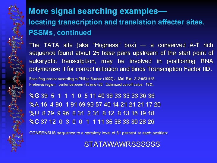
More signal searching examples— locating transcription and translation affecter sites. PSSMs, continued The TATA site (aka “Hogness” box) — a conserved A-T rich sequence found about 25 base pairs upstream of the start point of eukaryotic transcription, may be involved in positioning RNA polymerase II for correct initiation and binds Transcription Factor IID. Base freguencies according to Philipp Bucher (1990) J. Mol. Biol. 212: 563 -578. Biol. Preferred region: center between -36 and -20. Optimized cut-off value: 79%. %G 39 5 1 1 1 0 5 11 40 39 33 33 33 36 36 %A 16 4 90 1 91 69 93 57 40 14 21 21 21 17 20 %U 8 79 9 96 8 31 2 31 8 12 8 13 16 19 18 %C 37 12 0 3 0 0 1 1 11 35 38 33 30 28 26 CONSENSUS sequence to a certainty level of 61 percent at each position: STATAWAWRSSSSSS

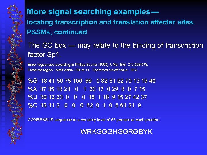
More signal searching examples— locating transcription and translation affecter sites. PSSMs, continued The GC box — may relate to the binding of transcription factor Sp 1. Base freguencies according to Philipp Bucher (1990) J. Mol. Biol. 212: 563 -578. Biol. Preferred region: motif within -164 to +1. Optimized cut-off value: 88%. %G %A %U %C 18 41 56 75 100 99 0 82 81 62 70 13 19 40 37 35 18 24 0 1 20 17 0 29 8 0 7 15 30 12 23 0 0 0 18 1 18 9 15 27 42 37 15 11 2 0 0 0 62 0 1 0 6 61 31 9 CONSENSUS sequence to a certainty level of 67 percent at each position: WRKGGGHGGRGBYK

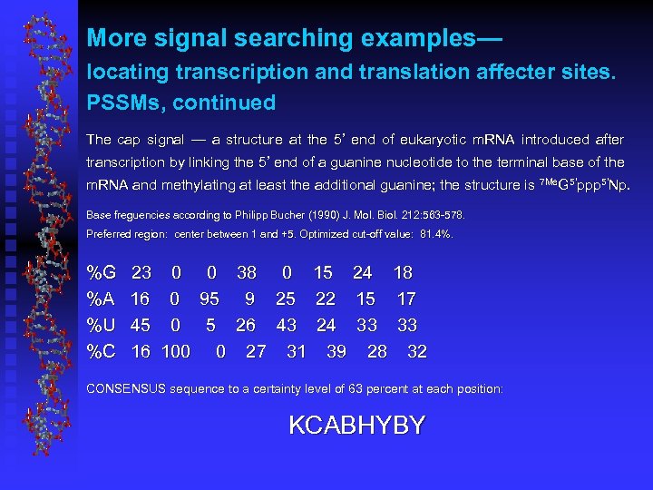
More signal searching examples— locating transcription and translation affecter sites. PSSMs, continued The cap signal — a structure at the 5’ end of eukaryotic m. RNA introduced after transcription by linking the 5’ end of a guanine nucleotide to the terminal base of the m. RNA and methylating at least the additional guanine; the structure is 7 Me. G 5’ppp 5’Np. Base freguencies according to Philipp Bucher (1990) J. Mol. Biol. 212: 563 -578. Biol. Preferred region: center between 1 and +5. Optimized cut-off value: 81. 4%. %G %A %U %C 23 0 16 0 45 0 16 100 0 38 0 15 24 18 95 9 25 22 15 17 5 26 43 24 33 33 0 27 31 39 28 32 CONSENSUS sequence to a certainty level of 63 percent at each position: KCABHYBY

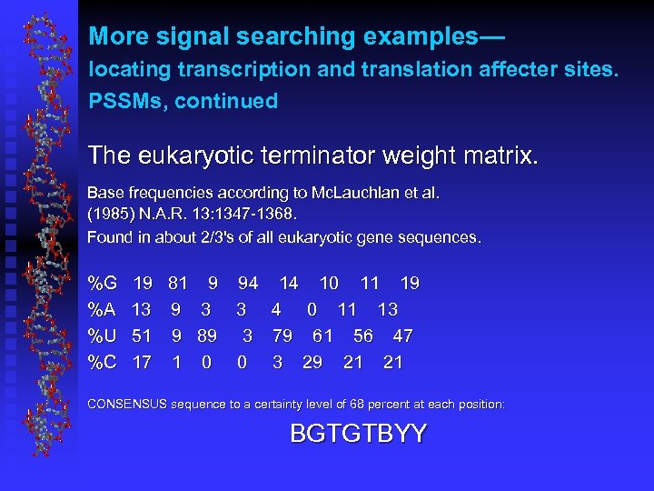
More signal searching examples— locating transcription and translation affecter sites. PSSMs, continued The eukaryotic terminator weight matrix. Base frequencies according to Mc. Lauchlan et al. (1985) N. A. R. 13: 1347 -1368. Found in about 2/3's of all eukaryotic gene sequences. %G %A %U %C 19 81 9 94 13 9 3 3 51 9 89 3 17 1 0 0 14 10 11 19 4 0 11 13 79 61 56 47 3 29 21 21 CONSENSUS sequence to a certainty level of 68 percent at each position: BGTGTBYY

And to extend the 2 D PSSM concept even further. . . Michael Gribskov envisioned special weight matrices in which conserved areas of the alignment receive the most importance, variable regions hardly matter, and gaps are variably weighted depending where they are! These are often called “profiles. ”

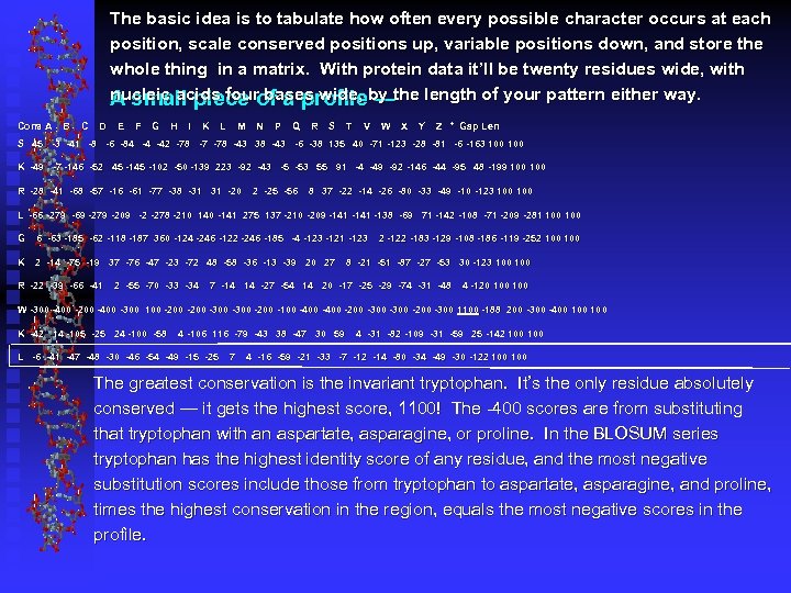
The basic idea is to tabulate how often every possible character occurs at each position, scale conserved positions up, variable positions down, and store the whole thing in a matrix. With protein data it’ll be twenty residues wide, with nucleic acids four bases wide, — A small piece of a profileby the length of your pattern either way. Cons A B C D E F G H I K L M N P Q R S T V W X Y Z * Gap Len S 45 -3 -41 -8 -6 -84 -4 -42 -78 -7 -78 -43 38 -43 -6 -38 135 40 -71 -123 -28 -81 -6 -163 100 K -49 -7 -146 -52 45 -102 -50 -139 223 -92 -43 -5 -53 55 91 -4 -49 -92 -146 -44 -95 48 -199 100 R -28 -41 -68 -57 -16 -61 -77 -38 -31 31 -20 2 -25 -56 8 37 -22 -14 -26 -80 -33 -49 -10 -123 100 L -66 -279 -69 -279 -209 -2 -278 -210 140 -141 275 137 -210 -209 -141 -138 -69 71 -142 -108 -71 -209 -281 100 G 6 -63 -185 -62 -118 -187 360 -124 -246 -122 -246 -185 -4 -123 -121 -123 K 2 -14 -75 -19 37 -76 -47 -23 -72 48 -58 -36 -13 -39 20 27 R -22 -39 -66 -41 2 -55 -70 -33 -34 2 -122 -183 -129 -108 -186 -119 -252 100 8 -21 -51 -87 -27 -53 30 -123 100 7 -14 14 -27 -54 14 20 -17 -25 -29 -74 -31 -48 4 -120 100 W -300 -400 -200 -400 -300 100 -200 -300 -200 -100 -400 -200 -300 1100 -188 200 -300 -400 100 K -42 14 -105 -25 24 -100 -58 4 -106 116 -79 -43 38 -47 30 59 L -6 -41 -47 -48 -30 -46 -54 -49 -15 -25 7 4 -31 -82 -109 -31 -59 25 -142 100 4 -16 -59 -21 -33 -7 -12 -14 -80 -34 -49 -30 -122 100 The greatest conservation is the invariant tryptophan. It’s the only residue absolutely conserved — it gets the highest score, 1100! The -400 scores are from substituting that tryptophan with an aspartate, asparagine, or proline. In the BLOSUM series tryptophan has the highest identity score of any residue, and the most negative substitution scores include those from tryptophan to aspartate, asparagine, and proline, times the highest conservation in the region, equals the most negative scores in the profile.

Some profile variations As powerful as ‘traditional’ Gribskov style profiles are, they require a lot of time and skill to prepare and validate, and they are heuristics based. Excess subjectivity and a lack of formal statistical rigor contribute as drawbacks. Sean Eddy developed the HMMer package, which uses Hidden Markov modeling, with a formal probabilistic basis and consistent gap insertion theory, to build and manipulate HMMer profiles and profile databases, to search sequences against HMMer profile databases and visa versa, and to easily create multiple sequence alignments using HMMer profiles as a ‘seed. ’

Profile variations, continued Bailey and Elkan’s Expectation Maximization (MEME) uses Bayesian probabilities and unsupervised learning to find, de novo, unknown conserved motifs among a group of unaligned, ungapped sequences. The motifs do not have to be in congruent order among the different sequences; i. e. it has the power to discover ‘unalignable’ motifs between sequences. This characteristic differentiates MEME from the other profile building techniques. It can be particularly effective in discovering regulatory elements in common between co-regulated genes.

What about those content approaches — strategies for finding coding regions based on the content of the DNA itself Searching by content utilizes the fact that genes necessarily have many implicit biological constraints imposed on their genetic code. This induces certain periodicities and patterns to produce distinctly unique coding sequences; non-coding stretches do not exhibit this type of periodic compositional bias. These principles can help discriminate structural genes in two ways: 1) based on the local “non-randomness” of a stretch, and 2) based on the known codon usage of a particular life form. The first, the non-randomness test, does not tell us anything about the particular strand or reading frame; however, it does not require a previously built codon usage table. The second approach is based on the fact that different organisms use different frequencies of codons to code for particular amino acids. This does require a codon usage table built up from known translations; however, it also tells us the strand reading frame for the gene products as opposed to the former.

“Non-randomness” content approaches — Rely solely on the base compositional bias of every third position base but does not tell us anything about the particular strand or reading frame; however, it does not require a previously built codon usage table. The plot is divided into three regions: top and bottom areas predict coding and noncoding regions, respectively, the middle area claims no statistical significance.

Codon usage content approaches — Genomes use synonymous codons unequally sorted phylogenetically. Requires a codon usage table built up from known translations; however, it also tells us the strand reading frame for the gene products. Each forward reading frame indicates a red codon preference curve and a blue third position GC bias curve.

Web servers for gene finding Many servers are available for help with gene finding analyses. Most combine many of the previousmethods but they consolidate the information and often combine signal and content methods with homology inference in order to ascertain exon locations. Many use powerful neural net or artificial intelligence approaches to assist in this difficult ‘decision’ process. A wonderful bibliography on computational methods for gene recognition has been compiled by Wentian Li (http: //www. nslij-genetics. org/gene/), and the Baylor College of Medicine’s Gene Feature Search (http: //searchlauncher. bcm. tmc. edu/seqsearch/gene-search. html) is another nice portal to several gene finding tools.

Genome scale analyses — map browsers try to tie it all together — Genetic linkage mapping databases for most large genome projects— H. sapiens, Mus, Drosophila, C. elegans, Saccharomyces, Arabidopsis, E. coli. . . usually link to other databases within the context of a genome browser or map viewer. Examples include: NCBI’s Map Viewer (http: //www. ncbi. nlm. nih. gov/mapview/), the Ensemble Project (http: //www. ensembl. org/), the UCSC Genome Browser at (http: //genome. ucsc. edu/), and the Lawrence Livermore National Laboratory ECR Browser (http: //www. dcode. org/).

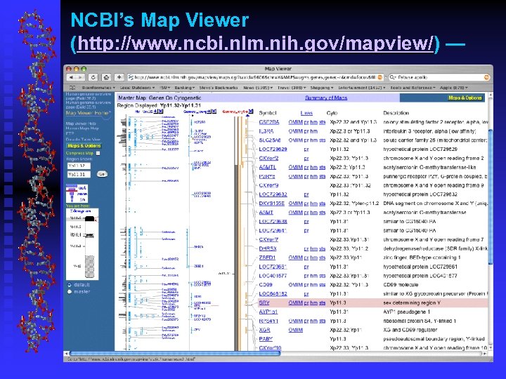
NCBI’s Map Viewer (http: //www. ncbi. nlm. nih. gov/mapview/) —

Sanger Center for Bio. Informatics Ensembl project (http: //www. ensembl. org/) —

University of California, Santa Cruz Genome Browser (http: //genome. ucsc. edu/) —

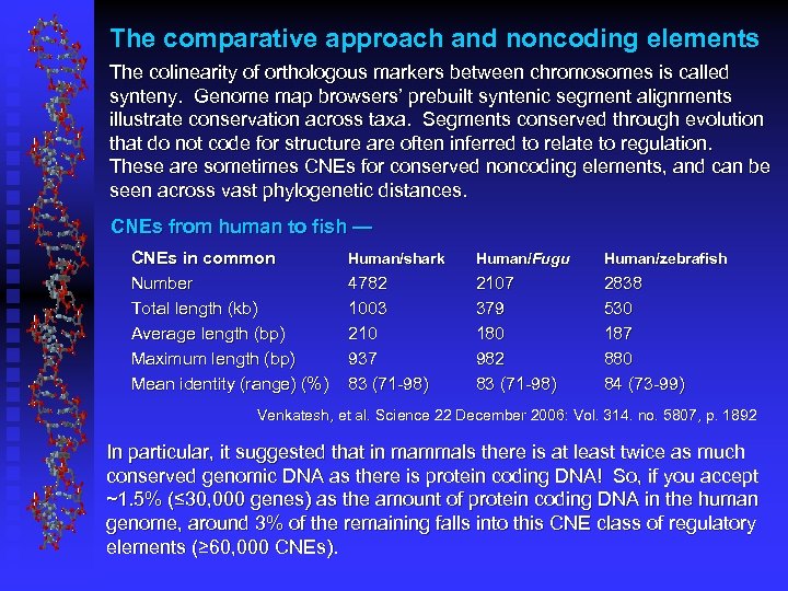
The comparative approach and noncoding elements The colinearity of orthologous markers between chromosomes is called synteny. Genome map browsers’ prebuilt syntenic segment alignments illustrate conservation across taxa. Segments conserved through evolution that do not code for structure are often inferred to relate to regulation. These are sometimes CNEs for conserved noncoding elements, and can be seen across vast phylogenetic distances. CNEs from human to fish — CNEs in common Number Total length (kb) Average length (bp) Maximum length (bp) Mean identity (range) (%) Human/shark Human/Fugu Human/zebrafish 4782 1003 210 937 83 (71 -98) 2107 379 180 982 83 (71 -98) 2838 530 187 880 84 (73 -99) Venkatesh, et al. Science 22 December 2006: Vol. 314. no. 5807, p. 1892 In particular, it suggested that in mammals there is at least twice as much conserved genomic DNA as there is protein coding DNA! So, if you accept ~1. 5% (≤ 30, 000 genes) as the amount of protein coding DNA in the human genome, around 3% of the remaining falls into this CNE class of regulatory elements (≥ 60, 000 CNEs).

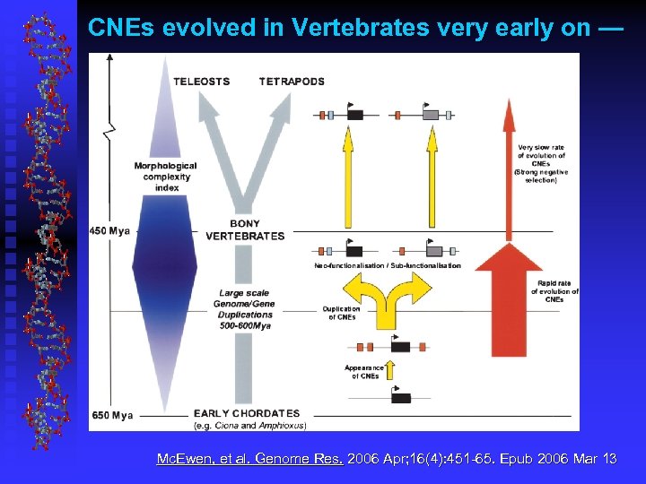
CNEs evolved in Vertebrates very early on — Mc. Ewen, et al. Genome Res. 2006 Apr; 16(4): 451 -65. Epub 2006 Mar 13

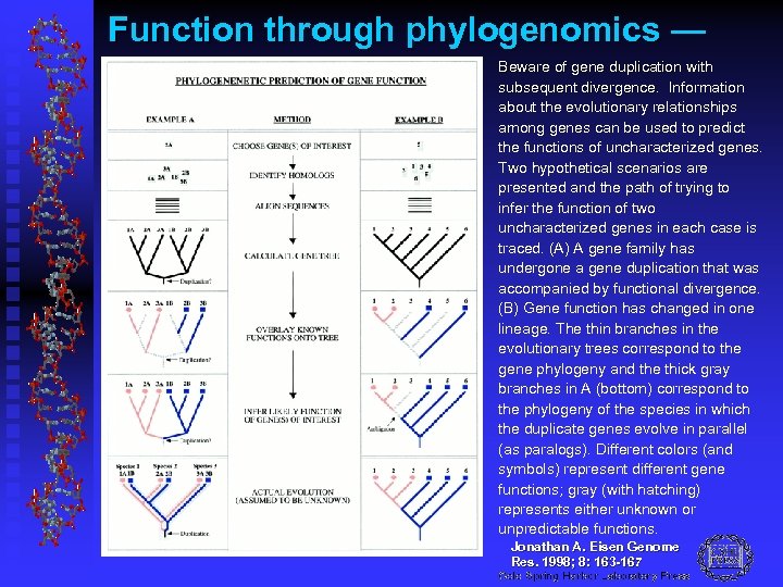
Function through phylogenomics — Beware of gene duplication with subsequent divergence. Information about the evolutionary relationships among genes can be used to predict the functions of uncharacterized genes. Two hypothetical scenarios are presented and the path of trying to infer the function of two uncharacterized genes in each case is traced. (A) A gene family has undergone a gene duplication that was accompanied by functional divergence. (B) Gene function has changed in one lineage. The thin branches in the evolutionary trees correspond to the gene phylogeny and the thick gray branches in A (bottom) correspond to the phylogeny of the species in which the duplicate genes evolve in parallel (as paralogs). Different colors (and symbols) represent different gene functions; gray (with hatching) represents either unknown or unpredictable functions. Jonathan A. Eisen Genome Res. 1998; 8: 163 -167

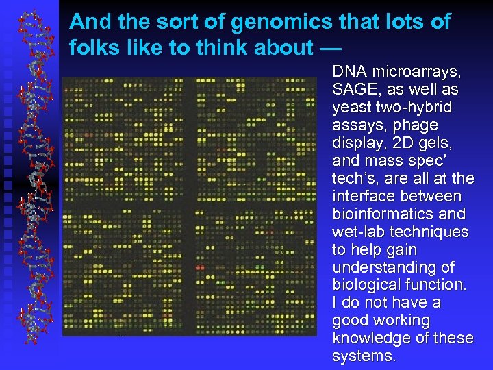
And the sort of genomics that lots of folks like to think about — DNA microarrays, SAGE, as well as yeast two-hybrid assays, phage display, 2 D gels, and mass spec’ tech’s, are all at the interface between bioinformatics and wet-lab techniques to help gain understanding of biological function. I do not have a good working knowledge of these systems.

Conclusions — There’s a bewildering assortment of bioinformatics databases and ways to access and manipulate the information within them. The key is to learn how to use the data and the methods in the most efficient manner! The better you understand the chemical, physical, and biological systems involved, the better your chance of success in analyzing them. Certain strategies are inherently more appropriate to others in certain circumstances. Making these types of subjective, discriminatory decisions is one of the most important ‘take-home’ messages I can offer! Gunnar von Heijne in his old but incredibly readable treatise, Sequence Analysis in Molecular Biology; Treasure Trove or Trivial Pursuit (1987), provides a very appropriate conclusion: “Think about what you’re doing; use your knowledge of the molecular system involved to guide both your interpretation of results and your direction of inquiry; use as much information as possible; and do not blindly accept everything the computer offers you. ” “. . . if any lesson is to be drawn. . . it surely is that to be able to make a useful contribution one must first and foremost be a biologist, and only second a theoretician. . We have to develop better algorithms, we have to find ways to cope with the massive amounts of data, and above all we have to become better biologists. But that’s all it takes. ”

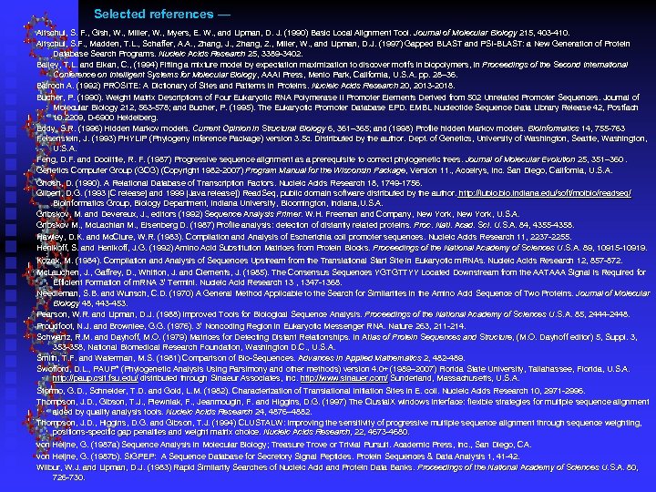
Selected references — Altschul, S. F. , Gish, W. , Miller, W. , Myers, E. W. , and Lipman, D. J. (1990) Basic Local Alignment Tool. Journal of Molecular Biology 215, 403 -410. Altschul, Gish, Lipman, Altschul, S. F. , Madden, T. L. , Schaffer, A. A. , Zhang, J. , Zhang, Z. , Miller, W. , and Lipman, D. J. (1997) Gapped BLAST and PSI-BLAST: a New Generation of Protein Altschul, Lipman, Database Search Programs. Nucleic Acids Research 25, 3389 -3402. Bailey, T. L. and Elkan, C. , (1994) Fitting a mixture model by expectation maximization to discover motifs in biopolymers, in Proceedings of the Second International Elkan, Conference on Intelligent Systems for Molecular Biology, AAAI Press, Menlo Park, California, U. S. A. pp. 28– 36. Biology, Bairoch A. (1992) PROSITE: A Dictionary of Sites and Patterns in Proteins. Nucleic Acids Research 20, 2013 -2018. Bucher, P. (1990). Weight Matrix Descriptions of Four Eukaryotic RNA Polymerase II Promoter Elements Derived from 502 Unrelated Promoter Sequences. Journal of Molecular Biology 212, 563 -578; and Bucher, P. (1995). The Eukaryotic Promoter Database EPD. EMBL Nucleotide Sequence Data Library Release 42, Postfach 10. 2209, D-6900 Heidelberg. Eddy, S. R. (1996) Hidden Markov models. Current Opinion in Structural Biology 6, 361– 365; and (1998) Profile hidden Markov models. Bioinformatics 14, 755 -763 Felsenstein, J. (1993) PHYLIP (Phylogeny Inference Package) version 3. 5 c. Distributed by the author. Dept. of Genetics, University of Washington, Seattle, Washington, Felsenstein, U. S. A. Feng, D. F. and Doolittle, R. F. (1987) Progressive sequence alignment as a prerequisite to correct phylogenetic trees. Journal of Molecular Evolution 25, 351– 360. Feng, Genetics Computer Group (GCG) (Copyright 1982 -2007) Program Manual for the Wisconsin Package, Version 11. , Accelrys, Inc. San Diego, California, U. S. A. Package, Accelrys, Ghosh, D. (1990). A Relational Database of Transcription Factors. Nucleic Acids Research 18, 1749 -1756. Gilbert, D. G. (1993 [C release] and 1999 [Java release]) Read. Seq, public domain software distributed by the author. http: //iubio. indiana. edu/soft/molbio/readseq/ Read. Seq, http: //iubio. indiana. Bioinformatics Group, Biology Department, Indiana University, Bloomington, Indiana, U. S. A. Gribskov, M. and Devereux, J. , editors (1992) Sequence Analysis Primer. W. H. Freeman and Company, New York, U. S. A. Gribskov, Primer. Gribskov M. , Mc. Lachlan M. , Eisenberg D. (1987) Profile analysis: detection of distantly related proteins. Proc. Natl. Acad. Sci. U. S. A. 84, 4355 -4358. Natl. Acad. Sci. Hawley, D. K. and Mc. Clure, W. R. (1983). Compilation and Analysis of Escherichia coli promoter sequences. Nucleic Acids Research 11, 2237 -2255. Henikoff, S. and Henikoff, J. G. (1992) Amino Acid Substitution Matrices from Protein Blocks. Proceedings of the National Academy of Sciences U. S. A. 89, 10915 -10919. Henikoff, Kozak, M. (1984). Compilation and Analysis of Sequences Upstream from the Translational Start Site in Eukaryotic m. RNAs. Nucleic Acids Research 12, 857 -872. Mc. Lauchen, J. , Gaffrey, D. , Whitton, J. and Clements, J. (1985). The Consensus Sequences YGTGTTYY Located Downstream from the AATAAA Signal is Required for Efficient Formation of m. RNA 3’ Termini. Nucleic Acid Research 13 , 1347 -1368. Needleman, S. B. and Wunsch, C. D. (1970) A General Method Applicable to the Search for Similarities in the Amino Acid Sequence of Two Proteins. Journal of Molecular Wunsch, Biology 48, 443 -453. Pearson, W. R. and Lipman, D. J. (1988) Improved Tools for Biological Sequence Analysis. Proceedings of the National Academy of Sciences U. S. A. 85, 2444 -2448. Lipman, Proudfoot, N. J. and Brownlee, G. G. (1976). 3’ Noncoding Region in Eukaryotic Messenger RNA. Nature 263, 211 -214. Schwartz, R. M. and Dayhoff, M. O. (1979) Matrices for Detecting Distant Relationships. In Atlas of Protein Sequences and Structure, (M. O. Dayhoff editor) 5, Suppl. 3, Dayhoff, Structure, Suppl. 353 -358, National Biomedical Research Foundation, Washington D. C. , U. S. A. Smith, T. F. and Waterman, M. S. (1981) Comparison of Bio-Sequences. Advances in Applied Mathematics 2, 482 -489. Swofford, D. L. , PAUP* (Phylogenetic Analysis Using Parsimony and other methods) version 4. 0+ (1989– 2007) Florida State University, Tallahassee, Florida, U. S. A. Swofford, http: //paup. csit. fsu. edu/ distributed through Sinaeur Associates, Inc. http: //www. sinauer. com/ Sunderland, Massachusetts, U. S. A. http: //paup. csit. fsu. http: //www. sinauer. com/ Stormo, G. D. , Schneider, T. D. and Gold, L. M. (1982). Characterization of Translational Initiation Sites in E. coli. Nucleic Acids Research 10, 2971 -2996. Thompson, J. D. , Gibson, T. J. , Plewniak, F. , Jeanmougin, F. and Higgins, D. G. (1997) The Clustal. X windows interface: flexible strategies for multiple sequence alignment Plewniak, Jeanmougin, aided by quality analysis tools. Nucleic Acids Research 24, 4876– 4882. Thompson, J. D. , Higgins, D. G. and Gibson, T. J. (1994) CLUSTALW: improving the sensitivity of progressive multiple sequence alignment through sequence weighting, positions-specific gap penalties and weight matrix choice. Nucleic Acids Research, 22, 4673 -4680. Research, von Heijne, G. (1987 a) Sequence Analysis in Molecular Biology; Treasure Trove or Trivial Pursuit. Academic Press, Inc. , San Diego, CA. von Heijne, G. (1987 b). SIGPEP: A Sequence Database for Secretory Signal Peptides. Protein Sequences & Data Analysis 1, 41 -42. Wilbur, W. J. and Lipman, D. J. (1983) Rapid Similarity Searches of Nucleic Acid and Protein Data Banks. Proceedings of the National Academy of Sciences U. S. A. 80, Lipman, 726 -730.