BINARY VARIABLES Qualitative Variables and in Multiple Linear

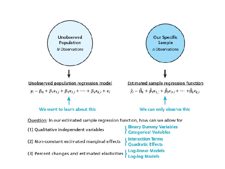
BINARY VARIABLES Qualitative Variables and in Multiple Linear Regression Analysis

Learning Objectives • Construct and use qualitative independent variables • Construct and use interaction effects • Construct and use qualitative dependent variables • Introduce and develop estimation techniques for Binary (limited) dependent variables • Introduce a simple non-linear regression model • Estimate a more fully-specified model

Construct and Use Qualitative Independent Variables • Qualitative explanatory variable (dummy variable) with two or more levels: – yes or no, on or off, male or female, race, geographic region of residence etc – coded as 0 or 1 • Regression intercepts are different if the variable is statistically significant (intercept dummy) • Assumes equal slopes for the other variables • The number of dummy variables needed is (number of levels - 1) – dummy variable trap

Dummy-Variable Model Example (with 2 Levels) Let: y = pie sales x 1 = price x 2 = holiday (X 2 = 1 if a holiday occurred during the week) (X 2 = 0 if there was no holiday that week)

Dummy-Variable Model Example (with 2 Levels) Continued Holiday No Holiday Different intercept y (sales) Holi da y No H o liday Same slope If H 0: β 2 = 0 is rejected, then “Holiday” has a significant effect on pie sales x 1 (Price)

• Most common use of dummy variables. • Modifies the regression model intercept parameter e. g. Let test the “location”, “location” model of real estate Suppose we take into account location near say a university or golf course

• P = βo + β 1 S +β 2 D + ε • S = square footage • D = dummy variable to represent if the characteristic is present or not (D is an intercept dummy variable) • D=1 • if property is in a desirable neighborhood 0 if not in a desirable neighborhood

• Effect of the dummy variable is best seen by examining the E(P). • If model is specified correctly, E(ε ) • =0 • E(P ) = ( βo + β 2 ) + β 1 S βo + β 1 S when D=1 when D = 0

Interpretation of the Dummy Variable Coefficient (with 2 Levels) Example: Sales: number of pies sold per week Price: pie price in $ 1 If a holiday occurred during the week Holiday: 0 If no holiday occurred = 15: on average, sales were 15 pies greater in weeks with a holiday than in weeks without a holiday, given the same price

In the real estate example • B 2 is the location premium in this case. • It is the difference between the Price of a house in a desirable are and one in a not so desirable area, all things held constant • The dummy variable is to capture the shift in the intercept as a result of some qualitative variable • D is an intercept dummy variable

• D is treated as any explanatory variable. • You can construct a confidence interval for B 2 • You can test if B 2 is significantly different from zero. • In such a test, if you accept Ho, then there is no difference between the two categories.

• Application of Intercept Dummy Variable • Wages = B 0 + B 1 Exp + B 2 Race +B 3 Gender + ε • Race = 1 if white 0 if non white Sex = 1 if male 0 if female Exp = job experience in years

Estimated regression • WAGES = 40, 000 + 1487 Exp + 1102 Race +1082 Gender Find: Mean salary for black female Mean salary for white male What ‘sucks’ more, being non-white or female? How would you go about testing if gender is significant in determining wages.

Determining the # of dummies to use • If h categories, then use h-1 dummies • Category left out defines reference group • If you use h dummies you’d fall into the dummy trap

Dummies for Multiple Categories • We can use dummy variables to control for something with multiple categories • Suppose everyone in your data is either a HS dropout, HS grad only, or college grad • To compare HS and college grads to HS dropouts, include 2 dummy variables • hsgrad = 1 if HS grad only, 0 otherwise; and colgrad = 1 if college grad, 0 otherwise 16

Multiple Categories (cont) • Any categorical variable can be turned into a set of dummy variables • Because the base group is represented by the intercept, if there are n categories there should be n – 1 dummy variables • If there a lot of categories, it may make sense to group some together • Example: top 10 ranking, 11 – 25, etc. 17

Dummy-Variable Models (more than 2 Levels) • The number of dummy variables is one less than the number of levels • Example: y = house price ; x 1 = square feet • The style of the house is also thought to matter: Style = ranch, split level, condo Three levels, so two dummy variables are needed

Dummy-Variable Models (more than 2 Levels) Continued Let the default category be “condo” shows the impact on price if the house is a ranch style, compared to a condo shows the impact on price if the house is a split level style, compared to a condo

Interpreting the Dummy Variable Coefficients (with 3 Levels) Suppose the estimated equation is For a condo: x 2 = x 3 = 0 For a ranch: x 3 = 0 For a split level: x 2 = 0 Same slope With the same square feet, a ranch will have an estimated average price of 23. 53 thousand dollars more than a condo and the intercept for a ranch is 20. 43 + 23. 53 = 43. 96 With the same square feet, a ranch will have an estimated average price of 18. 84 thousand dollars more than a condo and the intercept for a split level is 20. 43 + 19. 84 = 40. 27

Excel Example What type of relationship exists between energy use per capita and GDP per Capita. The initial regression is as follows: On average, if GDP per capita increases by $1000 US dollars, energy consumption per capita increases by. 07 tons. This is statistically significant at the 1% level.

Scatter Plots of this Relationship for Europe, North America, and South America Energy per Capita vs. GDP per Capita: Europe Energy per Capita vs. GDP per Capita: North America Energy per Capita (tons) 100 80 60 40 20 50 40 30 20 10 0 0 5 10 15 GDP per Capita ($1000 of US dollars) 20 5 10 15 GDP per Capita ($1000 of US dollars) Energy per Capita vs. GDP per Capita: South America Energy per Capita (tons) 120 3 2. 5 2 1. 5 1 0. 5 0 0 5 10 GDP per Capita ($1000 of US dollars) 15 Are the intercepts the same for these three locations? 20

Excel Example Are the intercepts different between Europe and North America with South America as the omitted group? On average, if GDP per capita increases by $1000 US dollars, energy consumption per capita increases by. 07 tons. This is statistically significant at the 10% level. The dummy variables for Europe and N. America are not statistically different from S. America at the 10% level.

Construct and Use Interaction Effects Interaction effects are the product of two different independent variables. We are first going to consider interaction effects between a quantitative variable and a dummy variable. (slope dummy) This type of interaction effect changes the slope of the quantitative variable for the various levels of the dummy variable.

Interactions Among Dummies • Interacting dummy variables is like subdividing the group • Example: have dummies for male, as well as hsgrad and colgrad • Add male*hsgrad and male*colgrad, for a total of 5 dummy variables –> 6 categories • Base group is female HS dropouts • hsgrad is for female HS grads, colgrad is for female college grads • The interactions reflect male HS grads and male college grads 25

Slope Dummy Variables • Allows for different slope in the relationship • Use an interaction variable between the actual variable and a dummy variable e. g. P = Bo + B 1 S+B 2(S*D)+ε D= 1 desirable area, 0 otherwise

• Captures the effect of location and size on the price of a house • E(P) = B 0 + (B 1+B 2)S if D=1 = B 0 + B 1 S if D = 0 in the desirable area, price per square foot is (B 1+B 2), and it is B 1 in other areas

If we believe that a house location affects both the intercept and the slope then the model is P = Bo + B 1 S+B 2(S*D)+B 3 D + ε

• Can also consider interacting a dummy variable, d, with a continuous variable, x • y = b 0 + d 1 d + b 1 x + d 2 d*x + u • If d = 0, then y = b 0 + b 1 x + u • If d = 1, then y = (b 0 + d 1) + (b 1+ d 2) x + u • This is interpreted as a change in the slope 29

Example of d 0 > 0 and d 1 < 0 y y = b 0 + b 1 x d=0 d=1 y = (b 0 + d 0 ) + (b 1 + d 1 ) x x 30

More on Dummy Interactions • Formally, the model is y = b 0 + d 1 male + d 2 hsgrad + d 3 colgrad + d 4 male*hsgrad + d 5 male*colgrad + b 1 x + u, then, for example: • If male = 0 and hsgrad = 0 and colgrad = 0 • y = b 0 + b 1 x + u • If male = 0 and hsgrad = 1 and colgrad = 0 • y = b 0 + d 2 hsgrad + b 1 x + u • If male = 1 and hsgrad = 0 and colgrad = 1 • y = b 0 + d 1 male + d 3 colgrad + d 5 male*colgrad + b 1 x + u 31

Interaction Regression Model Worksheet multiply x 1 by x 2 to get x 1 x 2, then run regression with y, x 1, x 2 , x 1 x 2

Consider the price of the house with three levels of the dummy variable Let the default category be “condo” and x 2 is 1 if ranch and 0 if not and x 3 is 1 if split level and 0 if not and x 1 is square feet. shows a change in the intercept on price if the house is a ranch style, compared to a condo shows a change in the intercept on price if the house is a split level style, compared to a condo shows the impact of the slope on price if the house is a ranch style, compared to a condo shows the impact of the slope on price if the house is a split level style, compared to a condo

Interaction Term Worksheet Suppose the estimated equation is

Visual Depiction of Interaction Terms with Dummy Variables

Excel Example Are the slopes and intercepts different between Europe and North America with South America as the omitted group? On average, if GDP per capita increases by $1000 US dollars, energy consumption per capita increases by. 07 tons. This is statistically significant at the 10% level. The dummy variables for Europe and N. America are not statistically different from S. America at the 10% level.

Control for Nonlinear Relationships • The relationship between the dependent variable and an independent variable may not be linear • Useful when scatter diagram indicates nonlinear relationship • Example: Quadratic model – – The second independent variable is the square of the first variable

Polynomial Regression Model General form: • where: β 0 = Population regression constant βi = Population regression coefficient for variable xj : j = 1, 2, …k p = Order of the polynomial i = Model error If p = 2 the model is a quadratic model:

Linear vs. Nonlinear Fit y y x x Linear fit does not give random residuals x x Nonlinear fit gives random residuals

Quadratic Regression Model Quadratic models may be considered when scatter diagram takes on the following shapes: y y β 1 < 0 β 2 > 0 x 1 y β 1 > 0 β 2 > 0 x 1 y β 1 < 0 β 2 < 0 β 1 = the coefficient of the linear term β 2 = the coefficient of the squared term x 1 β 1 > 0 β 2 < 0 x 1

Marginal Effect for the Quadratic Regression Model How does a one unit increase in xj affect the dependent variable y (the marginal effect)? This is just a partial derivative of y with respect to xj Notice that the effect that xj has on y changes depending on the value of xj and this should be evaluated at xj-1

Illustration of the Marginal Effect that xj has on y The marginal effect is the slope of a line tangent to the curve At x 1 j the marginal effect is positive At x 2 j the marginal effect is negative x 1 j x 2 j

Empirical Example of the Quadratic Effect: Utility Bill vs. Temperature Average Bill vs. Average Monthly Temperature $160. 00 $150. 00 $140. 00 Average Bill $130. 00 $120. 00 $110. 00 $100. 00 $90. 00 $80. 00 $70. 00 $60. 00 35 45 55 65 Average Monthly Temperature 75 85 95

Utility Bill vs. Temperature – Simple Linear Regression Even though the scatter plot shows a clear relationship between utility bill and temperature, there is no linear relationship between these two variables.

Utility Bill vs. Temperature – Quadratic Regression When a quadratic relationship is fit between utility bill and monthly temperature the linear and quadratic terms are now statistically significant at the 1% level.

Utility Bill vs. Temperature – Quadratic Regression Interpretation The marginal effect is The marginal effect at a temperature of 40 (evaluated at 39) is which means that if temperature increases from 39 to 40 degrees then the utility bill decreases by $5. 06. The marginal effect at a temperature of 80 (evaluated at 79) is which means that if temperature increases from 79 to 80 degrees then the utility bill increases by $2. 14.

Finding Where the Quadratic Function Reaches a Maximum (or Minimum) Method: Set the first derivative of the regression equal to 0 and solve for xj. or Using the utility bill example, the function reaches a minimum at or at a temperature of 67. 11 degrees. The function will reach a minimum if is positive and the function will reach a maximum if is negative.

Testing for Significance: Quadratic Model • Test for Overall Relationship between y and xj (test if the two parameters are jointly equal to 0). – Use an F-test with the Hypothesis H 0 : β 1 = β 2 = 0 (xj does not affect y) H 1: not H 0 (xj affects y) • Testing the Quadratic Effect – Compare quadratic model with the linear model – Use a t-test with the Hypothesis H 0 : β 2 = 0 (No 2 nd order polynomial term) H A : β 2 0 (2 nd order polynomial term is needed)

Higher Order Models y x If p = 3 the model is a cubic form:

Interaction Effects • Hypothesizes interaction between pairs of x variables – Response to one x variable varies at different levels of another x variable • Contains two-way cross product terms Basic Terms Interactive Terms

Effect of Interaction • Given: • Without interaction term, effect of x 1 on y is measured by β 1 • With interaction term, effect of x 1 on y is measured by β 1 + β 3 x 2 • Effect changes as x 2 increases

Evaluating Presence of Interaction • Hypothesize interaction between pairs of independent variables • Hypotheses: – H 0: β 3 = 0 (no interaction between x 1 and x 2) – HA: β 3 ≠ 0 (x 1 interacts with x 2)

Estimate Marginal Effects as Percent Changes and Elasticities The models are estimated taking natural logarithms of the dependent variable, the independent variable, or both. - Log-Linear Model - Log-Log Model

Log – Linear Model The population regression function is specified as and is interpreted as, “on average, if x 1 increases by 1 unit then y increases by Note that this is only an approximation because the natural log is a nonlinear function.

Empirical Example of the Log – Linear Model The dependent variable is the natural log of energy per capita This slope coefficient on gdppc is interpreted as, “on average, if GDP per capita increases by $1000 then energy consumption per capita goes up by (0. 026)100% or 2. 6%. ” This coefficient is statistically significant at the 1% level.

Empirical Example of the Log – Linear Model with Dummy Variables The dependent variable is the natural log of energy per capita with South America as the omitted group The Europe dummy variable coefficient is interpreted as “on average energy consumption per capita is 50. 5% higher in Europe than South America. ” The North America dummy variable coefficient is interpreted as “on average energy consumption per capita is 56. 6% higher in North America than South America. ” Europe is statistically insignificant while North America is marginally significant (significant at the 10% level).

Log – Log Model The population regression function is specified as and is interpreted as “on average, if x 1 increases by 1 percent then y increases by percent. ” In the log-log model is an elasticity.

Empirical Example of the Log – Log Model The dependent variable is the natural log of energy per capita This slope coefficient on lngdppc is interpreted as, “on average, if GDP per capita increases by 1% then energy consumption per capita goes up by. 69%. ” This coefficient is statistically significant at the 1% level.

Empirical Example of the Log – Linear Model with Dummy Variables The dependent variable is the natural log of energy per capita with South America as the omitted group The Europe dummy variable coefficient is interpreted as “on average energy consumption per capita is 9. 3% lower in Europe than South America. ” The North America dummy variable coefficient is interpreted as “on average energy consumption per capita is 41. 5% higher in North America than South America. ” Neither of these are statistically significant at the 10% level.