f2b58823729919b0e6291c30b3b8a19d.ppt
- Количество слайдов: 91

Bilevel Programming Approaches to Revenue Management and Price Setting Problems Gilles Savard, École Polytechnique de Montréal, GERAD, CRT Collaborators: P. Marcotte and C. Audet, L. Brotcorne, M. Gendreau, J. Gauvin, P. Hansen, A. Haurie, B. Jaumard, J. Judice, M. Labbé, D. Lavigne, R. Loulou, F. Semet, L. Vicente, D. J. White, D. Zhu Students: so many including J. -P. Côté, V. Rochon, A. Schoeb, É. Rancourt, F. Cirinei, M. Fortin, S. Roch, J. Guérin, S. Dewez, K. Lévy 16 janvier, 2004 Bilevel approaches to revenue management
Outline q. The revenue management problem q. The bilevel programming problem q. A price setting paradigm q… applied to toll setting q… a TSP instance q… applied to airline q. Conclusion 16 janvier, 2004 Bilevel approaches to revenue management
The revenue management problem q…the optimal revenue management of perishable assets through price segmentation (Weatherford and Bodily 92) q. Fixed (or almost) capacity q. Market segmentation q. Perishable products q. Presales q. High fixed cost q. Low variable cost 16 janvier, 2004 Bilevel approaches to revenue management
The revenue management problem RM Business process q. Forecasting q. Schedule with capacity q. Pricing q. Booking limits q. Seat sales 16 janvier, 2004 Bilevel approaches to revenue management
The revenue management problem Some issues in airline industry: q How to design the booking classes? q Restriction, min stay, max stay, service, etc… q … at what price? q Willingness to pay, competition, revenue, etc… q … how many tickets? q Given the evolution of sales (perishables) q … at what time? q Given the inventory and the date of flight 16 janvier, 2004 Bilevel approaches to revenue management
The revenue management problem Evolution of Pricing & RM q 1960’s: AA starts to use OR models for RM decisions q 1970’s: AA develops SABRE, providing automatic update of availability and prices q 1980’s: First RM software available q 1990’s: RM grows, even beyond airlines (hotel, rail, car rental, cruise, telecom, …) q 2000’s: networks 16 janvier, 2004 Bilevel approaches to revenue management
The revenue management problem Decision Support Tools focus on booking limits BUT mostly ignore pricing q. Complex problem: q. Must take into account its own action and the competition, as well as passenger behaviour q. Highly meshed network (hub-and-spoke) q. OD-based vs. Leg-based approach q. Data intensive 16 janvier, 2004 Bilevel approaches to revenue management
The revenue management problem q «Pricing has been ignored» P. Belobaba (MIT) q « Interest in RRM … is rising dramatically … RRM should be one of the top IT priorities for most retailers » AMR Research q «Pricing Decision Support Systems will spur the next round of airline productivity gains» L. Michaels (SH&E) 16 janvier, 2004 Bilevel approaches to revenue management
The revenue management problem q Until recently, capacity allocation and pricing were performed separately: capacity allocation is based on average historical prices; pricing is done without considering capacity. q However, there is a strong duality relationship between these two aspects. q A bilevel model combines both aspects while taking into account the topological structure of the network. 16 janvier, 2004 Bilevel approaches to revenue management
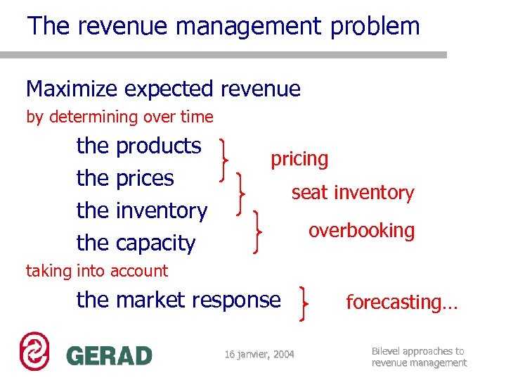
The revenue management problem Maximize expected revenue by determining over time the the products prices inventory capacity pricing seat inventory overbooking taking into account the market response 16 janvier, 2004 forecasting… Bilevel approaches to revenue management
Outline q. The revenue management problem q. The bilevel programming problem q. A price setting paradigm q… applied to toll setting q… a TSP instance q… applied to airline q. Conclusion 16 janvier, 2004 Bilevel approaches to revenue management
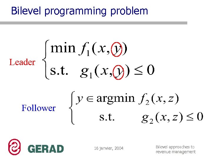
Bilevel programming problem Leader Follower 16 janvier, 2004 Bilevel approaches to revenue management
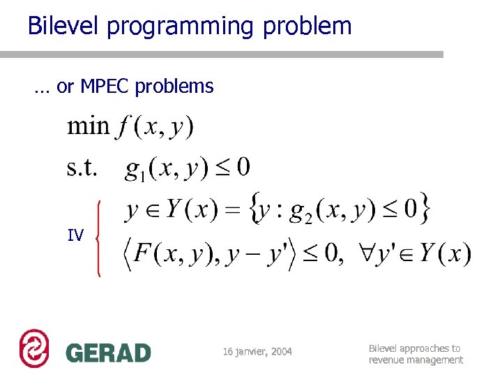
Bilevel programming problem … or MPEC problems IV 16 janvier, 2004 Bilevel approaches to revenue management
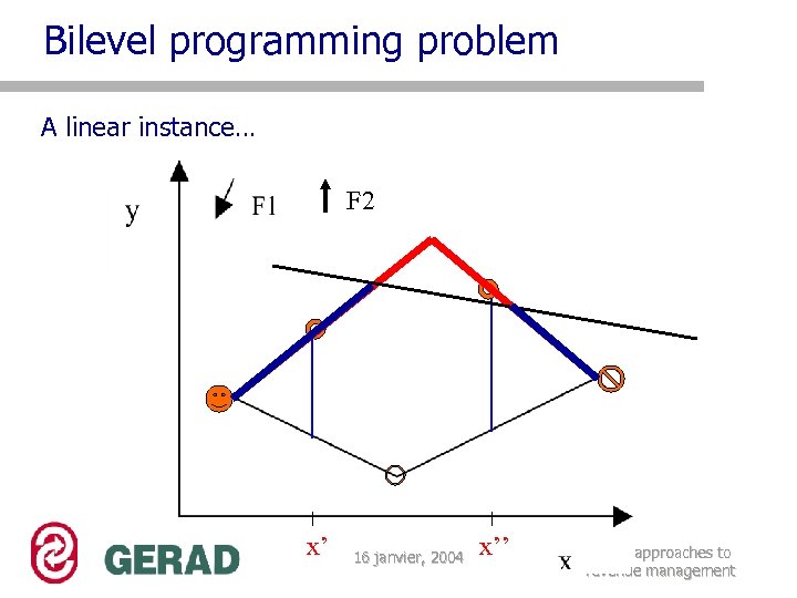
Bilevel programming problem A linear instance… F 2 x’ 16 janvier, 2004 x’’ Bilevel approaches to revenue management
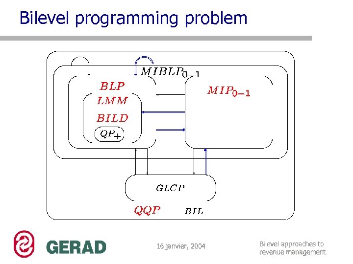
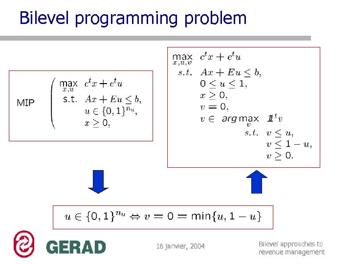
Bilevel programming problem q Typically non convex, disconnected and strongly NP-hard (HJS 92) (even for local optimality (VSJ 94)) q Optimal solution pareto solution (HSW 89, MS 91) q Steepest descent: BLP linear/quadratic (SG 93) q Many instances: q. Linear/linear (HJS 92, JF 90, BM 90) q. Linear/quadratic (BM 92) q. Convex/quadratic (JJS 96) q. Bilinear/bilinear (BD 02, LMS 98, BLMS 01) q. Bilinear/convex q. Convex/convex 16 janvier, 2004 Bilevel approaches to revenue management
Bilevel programming problem 16 janvier, 2004 Bilevel approaches to revenue management
Bilevel programming problem 16 janvier, 2004 Bilevel approaches to revenue management
Bilevel programming model q. Resolution approaches q. Combinatorial approaches (global solution) q. Lower level structure: combinatorial structure q. Descent approaches (on the bilevel model) q. Sensitivity analysis (local approach) (Outrata+Zowe) q. Descent approaches (on an approximated one -level model) q. Model still non convex (e. g. penalization of the second level KKT conditions) (Scholtes+Stöhr) 16 janvier, 2004 Bilevel approaches to revenue management
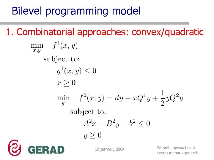
Bilevel programming model 1. Combinatorial approaches: convex/quadratic 16 janvier, 2004 Bilevel approaches to revenue management
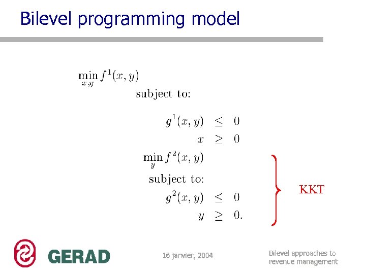
Bilevel programming model KKT 16 janvier, 2004 Bilevel approaches to revenue management
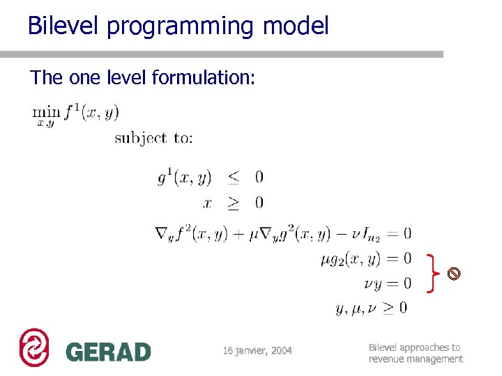
Bilevel programming model The one level formulation: 16 janvier, 2004 Bilevel approaches to revenue management
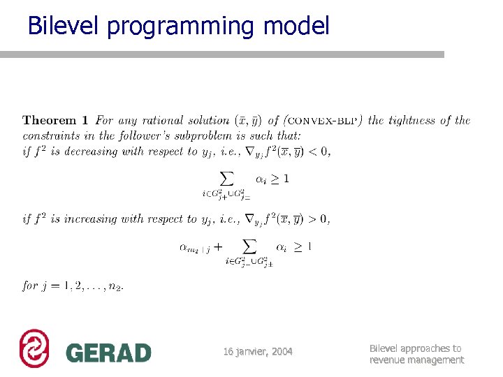
Bilevel programming model 16 janvier, 2004 Bilevel approaches to revenue management
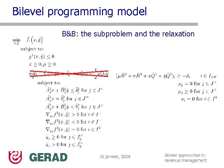
Bilevel programming model B&B: the subproblem and the relaxation 16 janvier, 2004 Bilevel approaches to revenue management

Bilevel programming model q An efficient B&B algorithm can be developed by q. Exploiting the monotonicity principle q. Using two subproblems (primal and dual) to drive the selection of the constraints q. Efficient separation schemes q. Using degradation estimation by penalties q. Using cuts q Size (exact solution): 60 x 60 to 300 X 150 q Heuristics: 600 x 600 (tabou, pareto) 16 janvier, 2004 Bilevel approaches to revenue management
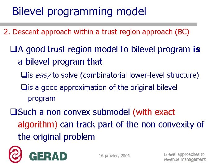
Bilevel programming model 2. Descent approach within a trust region approach (BC) q A good trust region model to bilevel program is a bilevel program that qis easy to solve (combinatorial lower-level structure) qis a good approximation of the original bilevel program q Such a non convex submodel (with exact algorithm) can track part of the non convexity of the original problem 16 janvier, 2004 Bilevel approaches to revenue management
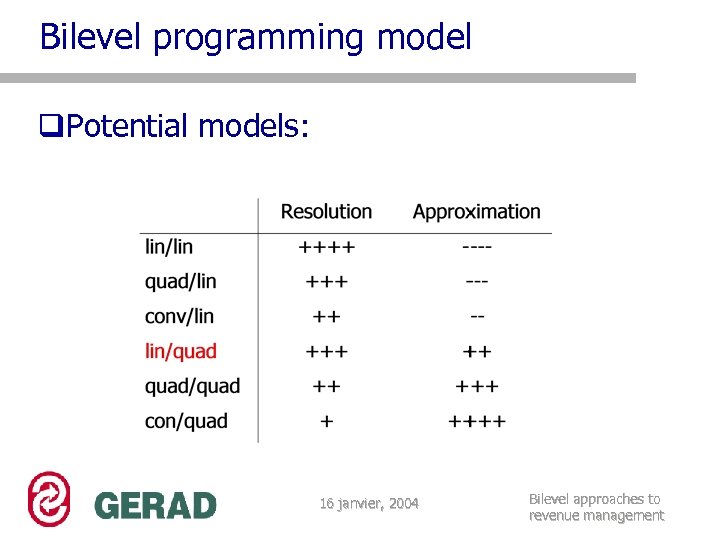
Bilevel programming model q. Potential models: 16 janvier, 2004 Bilevel approaches to revenue management
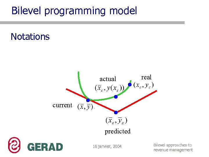
Bilevel programming model Notations actual real current predicted 16 janvier, 2004 Bilevel approaches to revenue management
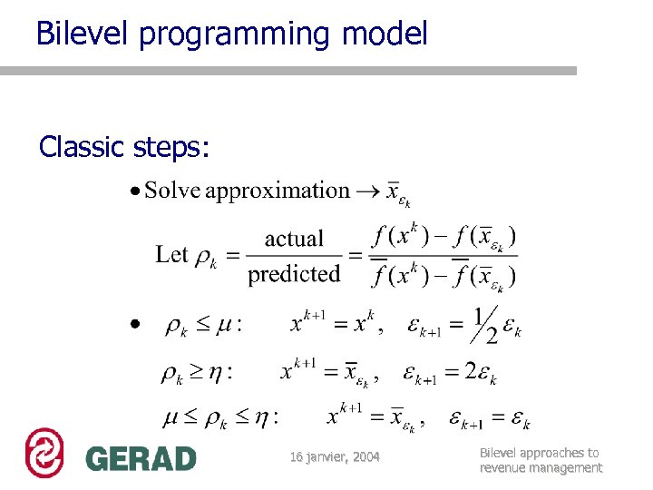
Bilevel programming model Classic steps: 16 janvier, 2004 Bilevel approaches to revenue management

Bilevel programming model With a linesearch step (to guaranty a strong stationary point) 16 janvier, 2004 Bilevel approaches to revenue management

Bilevel programming model b-stationary convergence 16 janvier, 2004 Bilevel approaches to revenue management
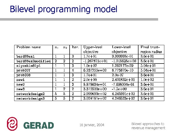
Bilevel programming model 16 janvier, 2004 Bilevel approaches to revenue management
Outline q. The revenue management problem q. The bilevel programming problem q. A price setting paradigm q… applied to toll setting q… a TSP instance q… applied to airline q. Conclusion 16 janvier, 2004 Bilevel approaches to revenue management
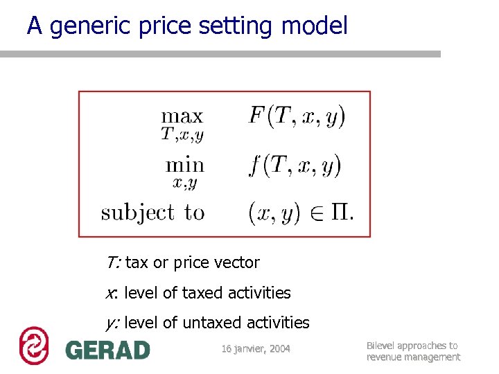
A generic price setting model T: tax or price vector x: level of taxed activities y: level of untaxed activities 16 janvier, 2004 Bilevel approaches to revenue management
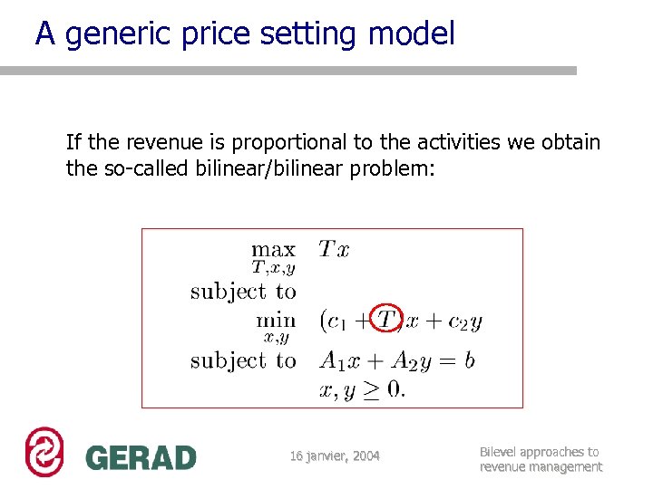
A generic price setting model If the revenue is proportional to the activities we obtain the so-called bilinear/bilinear problem: 16 janvier, 2004 Bilevel approaches to revenue management
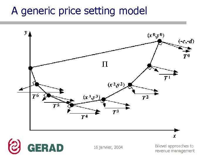
A generic price setting model 16 janvier, 2004 Bilevel approaches to revenue management
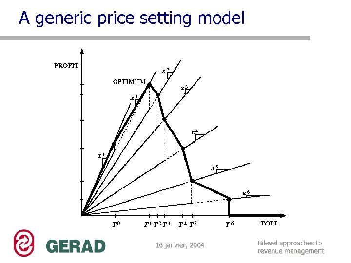
A generic price setting model 16 janvier, 2004 Bilevel approaches to revenue management
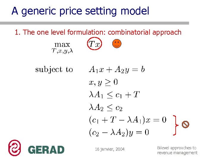
A generic price setting model 1. The one level formulation: combinatorial approach 16 janvier, 2004 Bilevel approaches to revenue management
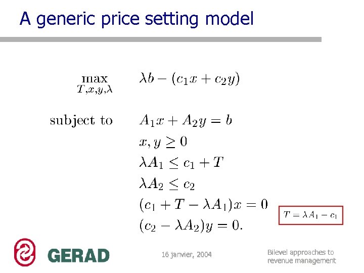
A generic price setting model 16 janvier, 2004 Bilevel approaches to revenue management
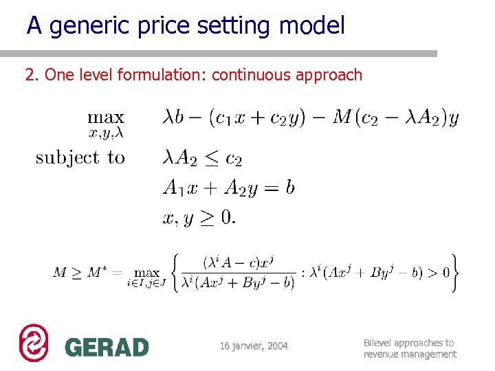
A generic price setting model 2. One level formulation: continuous approach 16 janvier, 2004 Bilevel approaches to revenue management
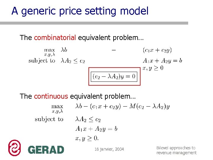
A generic price setting model The combinatorial equivalent problem… The continuous equivalent problem… 16 janvier, 2004 Bilevel approaches to revenue management
Outline q. The revenue management problem q. The bilevel programming problem q. A price setting paradigm q… applied to toll setting q… a TSP instance q… applied to airline q. Conclusion 16 janvier, 2004 Bilevel approaches to revenue management
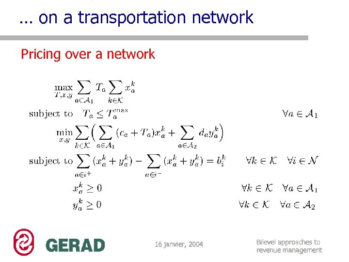
… on a transportation network Pricing over a network 16 janvier, 2004 Bilevel approaches to revenue management
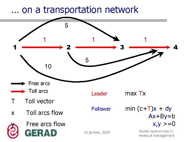
… on a transportation network 5 1 1 10 Free arcs Toll arcs T 1 2 Toll arcs flow y 4 5 Leader max Tx Follower min (c+T)x + dy Ax+By=b x, y >=0 16 janvier, 2004 Bilevel approaches to revenue management Toll vector x 3 1 Free arcs flow
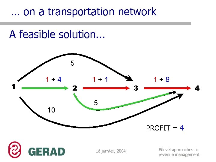
… on a transportation network A feasible solution. . . 5 1 1+4 10 2 1+1 3 1+8 4 5 PROFIT = 4 16 janvier, 2004 Bilevel approaches to revenue management
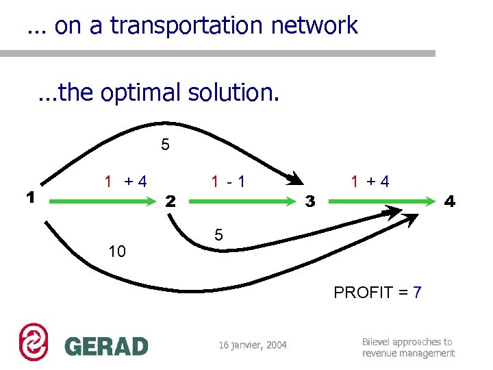
… on a transportation network …the optimal solution. 5 1 1 +4 10 2 1 -1 3 1 +4 4 5 PROFIT = 7 16 janvier, 2004 Bilevel approaches to revenue management
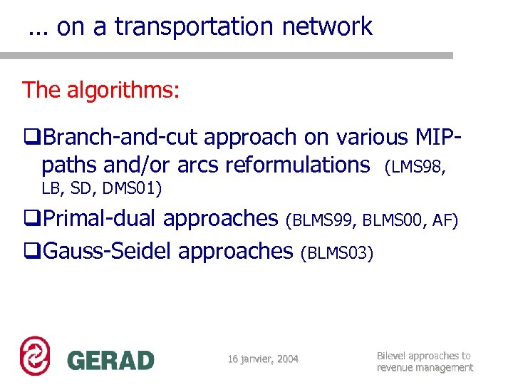
… on a transportation network The algorithms: q. Branch-and-cut approach on various MIPpaths and/or arcs reformulations (LMS 98, LB, SD, DMS 01) q. Primal-dual approaches (BLMS 99, BLMS 00, AF) q. Gauss-Seidel approaches (BLMS 03) 16 janvier, 2004 Bilevel approaches to revenue management
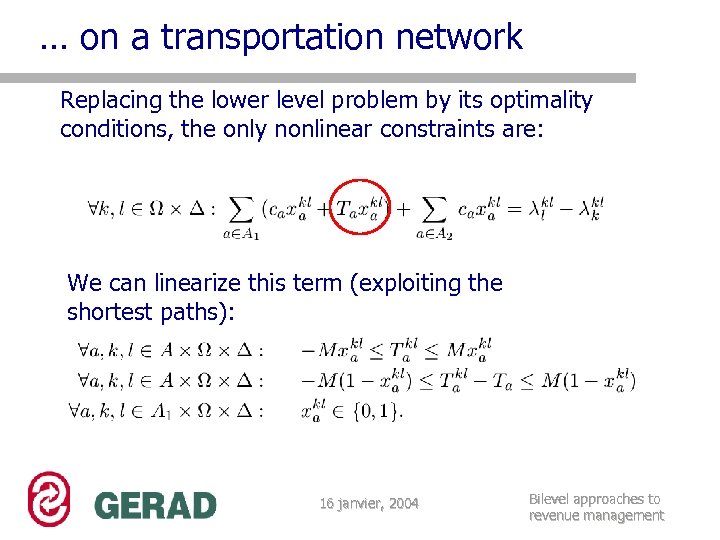
… on a transportation network Replacing the lower level problem by its optimality conditions, the only nonlinear constraints are: We can linearize this term (exploiting the shortest paths): 16 janvier, 2004 Bilevel approaches to revenue management
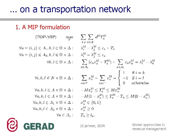
… on a transportation network 1. A MIP formulation 16 janvier, 2004 Bilevel approaches to revenue management
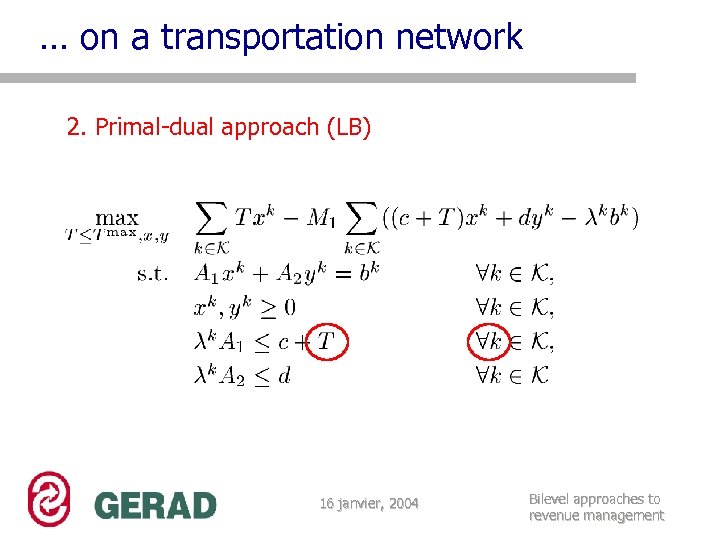
… on a transportation network 2. Primal-dual approach (LB) 16 janvier, 2004 Bilevel approaches to revenue management
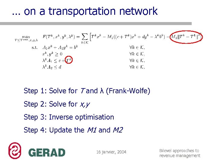
… on a transportation network Step 1: Solve for T and λ (Frank-Wolfe) Step 2: Solve for x, y Step 3: Inverse optimisation Step 4: Update the M 1 and M 2 16 janvier, 2004 Bilevel approaches to revenue management
Outline q. The revenue management problem q. The bilevel programming problem q. A price setting paradigm q… a toll setting problem q… a TSP instance q… applied to airline q. Conclusion 16 janvier, 2004 Bilevel approaches to revenue management

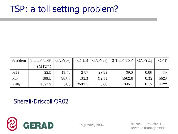
TSP: a toll setting problem? TSP: given a graph G=(V, E) and the length vector c, find a tour that minimizes the total length. 16 janvier, 2004 Bilevel approaches to revenue management
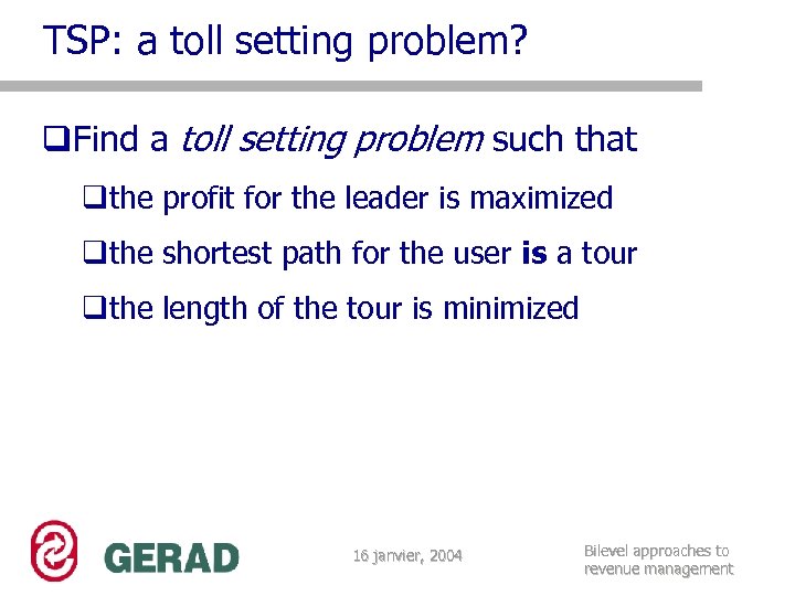
TSP: a toll setting problem? q. Find a toll setting problem such that qthe profit for the leader is maximized qthe shortest path for the user is a tour qthe length of the tour is minimized 16 janvier, 2004 Bilevel approaches to revenue management
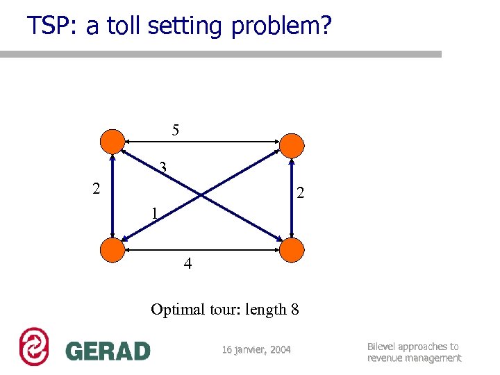
TSP: a toll setting problem? 5 3 2 2 1 4 Optimal tour: length 8 16 janvier, 2004 Bilevel approaches to revenue management
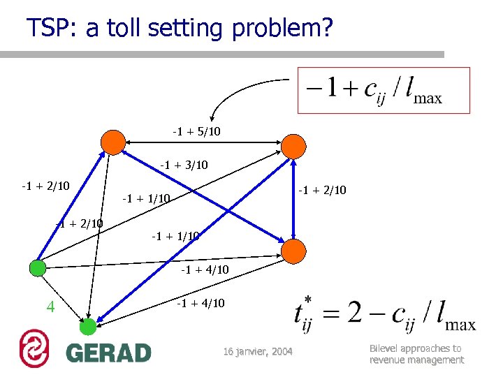
TSP: a toll setting problem? -1 + 5/10 -1 + 3/10 -1 + 2/10 -1 + 1/10 -1 + 4/10 4 -1 + 4/10 16 janvier, 2004 Bilevel approaches to revenue management
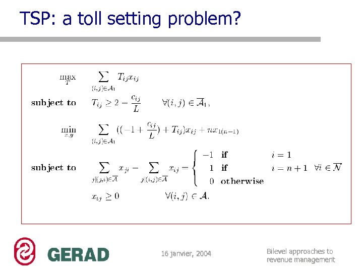
TSP: a toll setting problem? 16 janvier, 2004 Bilevel approaches to revenue management
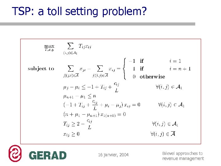
TSP: a toll setting problem? 16 janvier, 2004 Bilevel approaches to revenue management
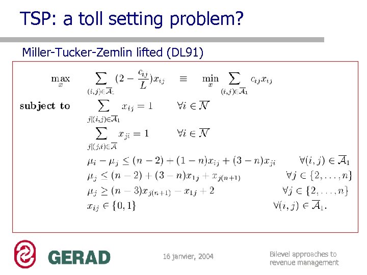
TSP: a toll setting problem? Miller-Tucker-Zemlin lifted (DL 91) 16 janvier, 2004 Bilevel approaches to revenue management
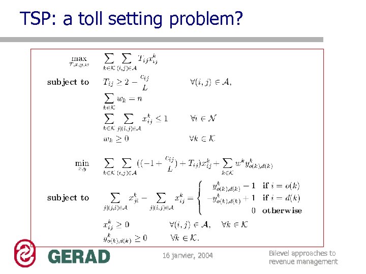
TSP: a toll setting problem? 16 janvier, 2004 Bilevel approaches to revenue management
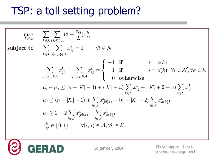
TSP: a toll setting problem? 16 janvier, 2004 Bilevel approaches to revenue management
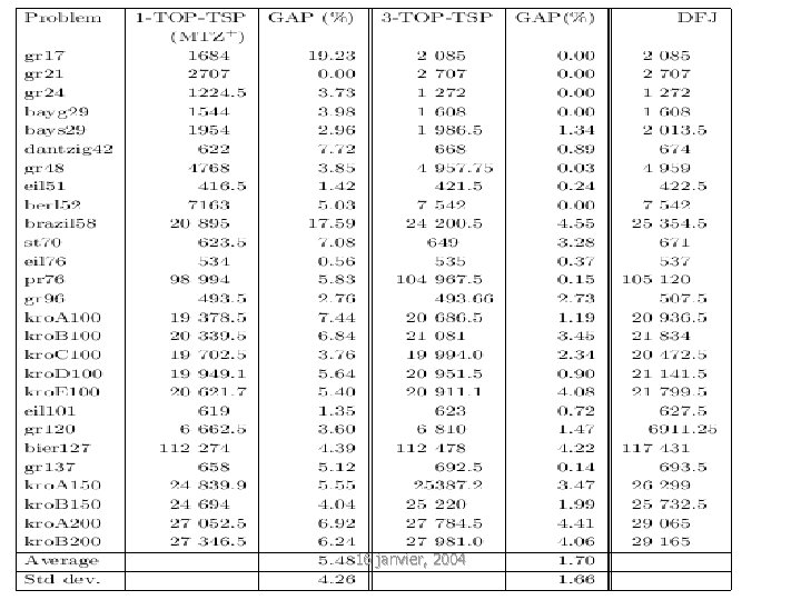
3. TSP: a toll setting problem? 16 janvier, 2004 Bilevel approaches to revenue management
TSP: a toll setting problem? Sherali-Driscoll OR 02 16 janvier, 2004 Bilevel approaches to revenue management
Outline q. The revenue management problem q. The bilevel programming problem q. A price setting paradigm q… applied to toll setting q… applied to telecommunication q… applied to airline q. Conclusion 16 janvier, 2004 Bilevel approaches to revenue management
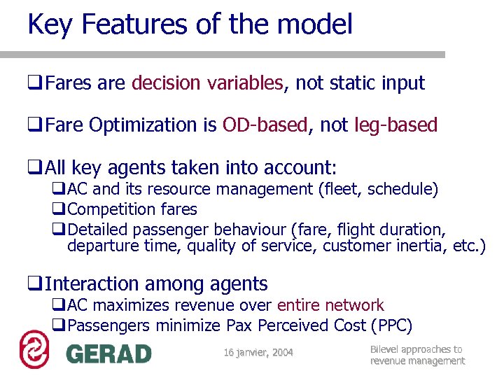
Key Features of the model q Fares are decision variables, not static input q Fare Optimization is OD-based, not leg-based q All key agents taken into account: q. AC and its resource management (fleet, schedule) q. Competition fares q. Detailed passenger behaviour (fare, flight duration, departure time, quality of service, customer inertia, etc. ) q Interaction among agents q. AC maximizes revenue over entire network q. Passengers minimize Pax Perceived Cost (PPC) 16 janvier, 2004 Bilevel approaches to revenue management
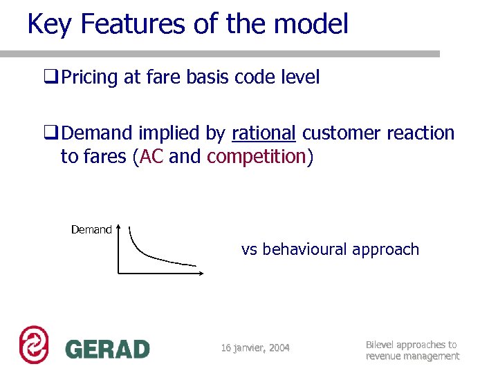
Key Features of the model q Pricing at fare basis code level q Demand implied by rational customer reaction to fares (AC and competition) Demand vs behavioural approach 16 janvier, 2004 Bilevel approaches to revenue management
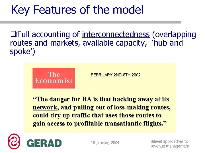
Key Features of the model q. Full accounting of interconnectedness (overlapping routes and markets, available capacity, ‘hub-andspoke’) FEBRUARY 2 ND-8 TH 2002 “The danger for BA is that hacking away at its network, and pulling out of loss-making routes, could dry up traffic that uses those routes to gain access to profitable transatlantic flights. ” 16 janvier, 2004 Bilevel approaches to revenue management
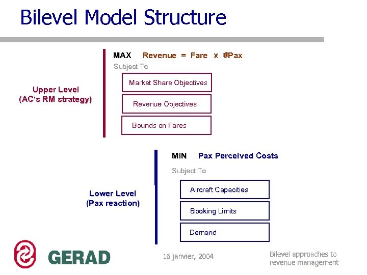
Bilevel Model Structure MAX Revenue = Fare X #Pax Subject To Upper Level (AC‘s RM strategy) Market Share Objectives Revenue Objectives Bounds on Fares MIN Pax Perceived Costs Subject To Lower Level (Pax reaction) Aircraft Capacities Booking Limits Demand 16 janvier, 2004 Bilevel approaches to revenue management
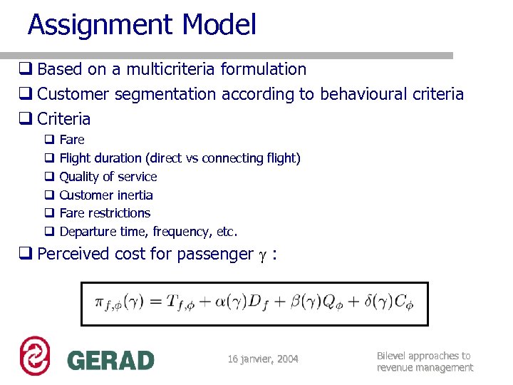
Assignment Model q Based on a multicriteria formulation q Customer segmentation according to behavioural criteria q Criteria q q q Fare Flight duration (direct vs connecting flight) Quality of service Customer inertia Fare restrictions Departure time, frequency, etc. q Perceived cost for passenger : 16 janvier, 2004 Bilevel approaches to revenue management
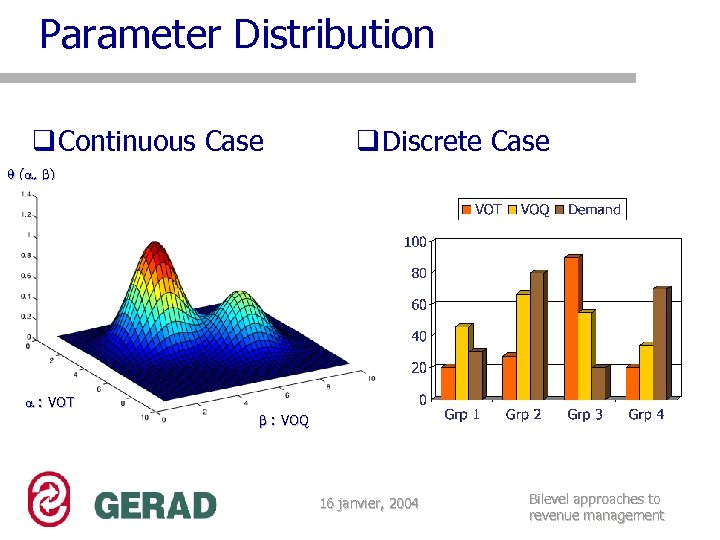
Parameter Distribution q Continuous Case q Discrete Case ( , ) : VOT : VOQ 16 janvier, 2004 Bilevel approaches to revenue management
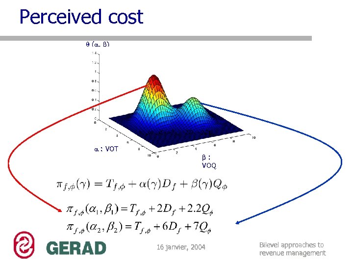
Perceived cost ( , ) : VOT : VOQ 16 janvier, 2004 Bilevel approaches to revenue management
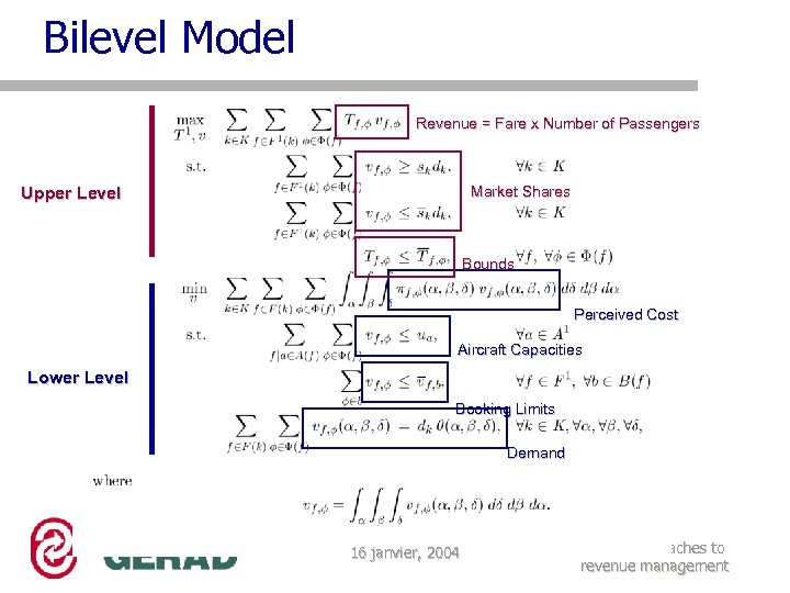
Bilevel Model Revenue = Fare x Number of Passengers Market Shares Upper Level Bounds Perceived Cost Aircraft Capacities Lower Level Booking Limits Demand 16 janvier, 2004 Bilevel approaches to revenue management
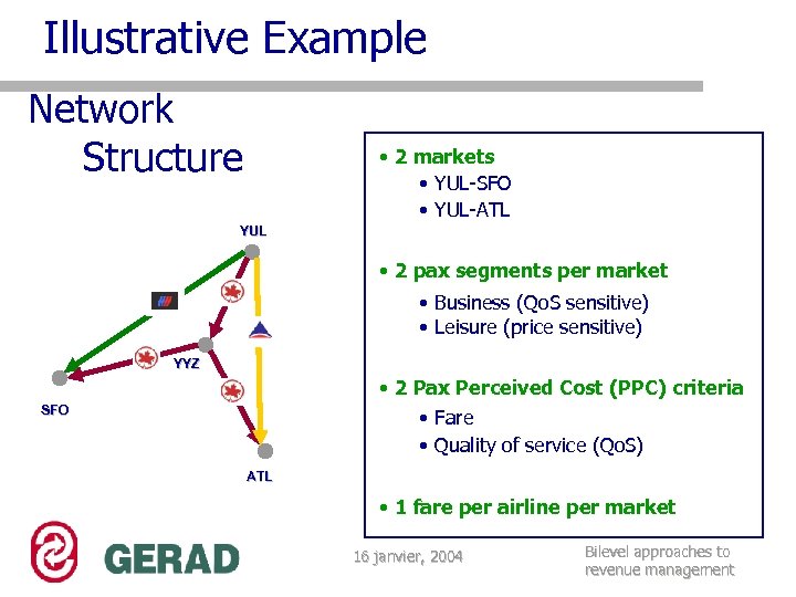
Illustrative Example Network Structure • 2 markets • YUL-SFO • YUL-ATL YUL • 2 pax segments per market • Business (Qo. S sensitive) • Leisure (price sensitive) YYZ • 2 Pax Perceived Cost (PPC) criteria • Fare • Quality of service (Qo. S) SFO ATL • 1 fare per airline per market 16 janvier, 2004 Bilevel approaches to revenue management
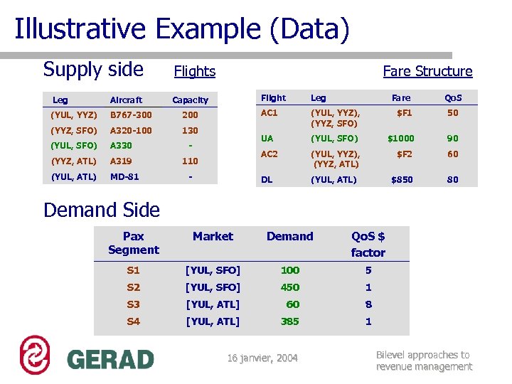
Illustrative Example (Data) Supply side Flights Fare Structure Aircraft (YUL, YYZ) B 767 -300 A 320 -100 (YUL, SFO) A 330 - (YYZ, ATL) A 319 110 (YUL, ATL) MD-81 - $F 1 50 (YUL, SFO) $1000 90 AC 2 130 (YUL, YYZ), (YYZ, SFO) UA Capacity Leg AC 1 200 (YYZ, SFO) Flight (YUL, YYZ), (YYZ, ATL) $F 2 60 DL Leg Fare Qo. S (YUL, ATL) $850 80 Demand Side Pax Segment Market Demand Qo. S $ factor S 1 [YUL, SFO] 100 5 S 2 [YUL, SFO] 450 1 S 3 [YUL, ATL] 60 8 S 4 [YUL, ATL] 385 1 16 janvier, 2004 Bilevel approaches to revenue management
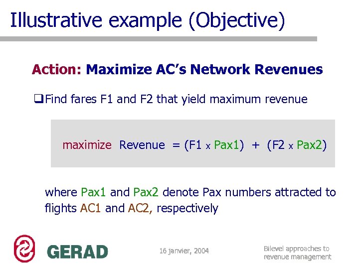
Illustrative example (Objective) Action: Maximize AC’s Network Revenues q. Find fares F 1 and F 2 that yield maximum revenue maximize Revenue = (F 1 x Pax 1) + (F 2 x Pax 2) where Pax 1 and Pax 2 denote Pax numbers attracted to flights AC 1 and AC 2, respectively 16 janvier, 2004 Bilevel approaches to revenue management
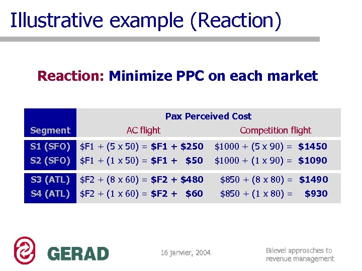
Illustrative example (Reaction) Reaction: Minimize PPC on each market Pax Perceived Cost Segment AC flight S 1 (SFO) $F 1 + (5 x 50) = $F 1 + $250 $1000 + (5 x 90) = $1450 S 2 (SFO) $F 1 + (1 x 50) = $F 1 + $50 $1000 + (1 x 90) = $1090 S 3 (ATL) $F 2 + (8 x 60) = $F 2 + $480 $850 + (8 x 80) = $1490 S 4 (ATL) $F 2 + (1 x 60) = $F 2 + $60 $850 + (1 x 80) = 16 janvier, 2004 Competition flight $930 Bilevel approaches to revenue management
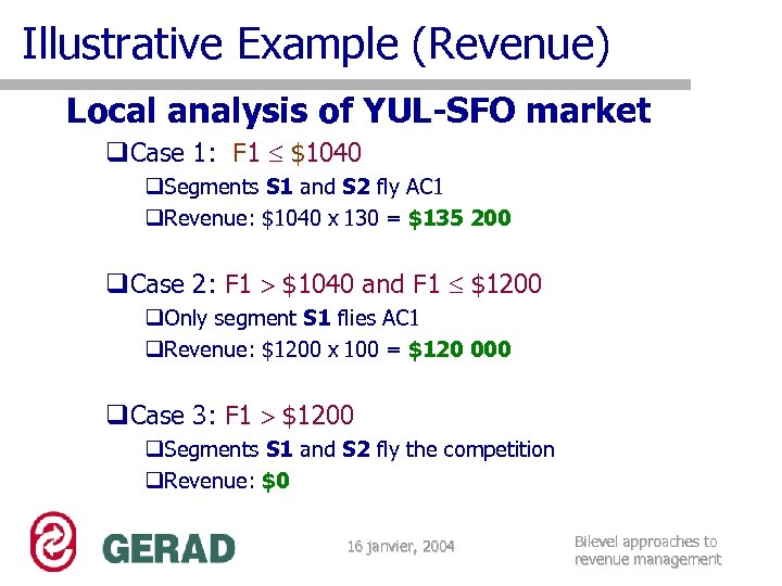
Illustrative Example (Revenue) Local analysis of YUL-SFO market q. Case 1: F 1 $1040 q. Segments S 1 and S 2 fly AC 1 q. Revenue: $1040 x 130 = $135 200 q. Case 2: F 1 $1040 and F 1 $1200 q. Only segment S 1 flies AC 1 q. Revenue: $1200 x 100 = $120 000 q. Case 3: F 1 $1200 q. Segments S 1 and S 2 fly the competition q. Revenue: $0 16 janvier, 2004 Bilevel approaches to revenue management
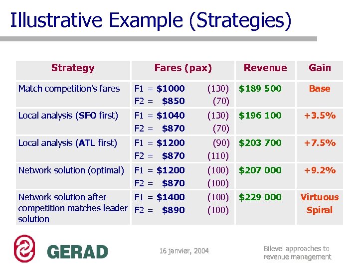
Illustrative Example (Strategies) Strategy Fares (pax) Revenue Gain Match competition’s fares F 1 = $1000 F 2 = $850 (130) (70) $189 500 Base Local analysis (SFO first) F 1 = $1040 F 2 = $870 (130) (70) $196 100 +3. 5% Local analysis (ATL first) F 1 = $1200 F 2 = $870 (90) (110) $203 700 +7. 5% Network solution (optimal) F 1 = $1200 F 2 = $870 (100) $207 000 +9. 2% Network solution after F 1 = $1400 competition matches leader F 2 = $890 solution (100) $229 000 Virtuous Spiral 16 janvier, 2004 Bilevel approaches to revenue management
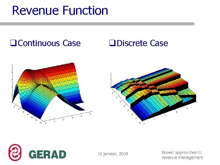
Revenue Function q Continuous Case q Discrete Case 16 janvier, 2004 Bilevel approaches to revenue management
Real-life Instance q. Thousands of O-D pairs (markets) q. More than 20 fare basis codes per market q. Hundreds of legs per day q. Hub-and-spoke structure q. Highly meshed network q. Extended planning horizon q. Capacity 16 janvier, 2004 Bilevel approaches to revenue management
Model Resolution q Discrete approach q Combinatorial heuristics q Branch-and-cut exact algorithms q Continuous approach q Sub-gradient based ascent method q Hybrid approach q Phase 1: coarse discrete approximation q Phase 2: further optimization (fine tuning) 16 janvier, 2004 Bilevel approaches to revenue management

Parameter Calibration q Procedure based on Hierarchical Inverse Optimization q Estimation from historical data q Same order of complexity (NP-Hard) q Calibration performed off-line on a regular basis 16 janvier, 2004 Bilevel approaches to revenue management
Issues q Continuous vs. discrete q Design of decomposition techniques to deal with the curse of dimensionality q Extremal solutions vs discretization q The dynamic of the process q Interaction with databases q Live scenarios 16 janvier, 2004 Bilevel approaches to revenue management
Conclusion q. Bilevel programming is a rich class of problems q. Interests in both theoretical and practical issues q. Keeping the structure and the meaning of the model of each agent q. The natural way of modeling the yield management problem 16 janvier, 2004 Bilevel approaches to revenue management
Additional Material 16 janvier, 2004 Bilevel approaches to revenue management
Bilevel programming model 16 janvier, 2004 Bilevel approaches to revenue management
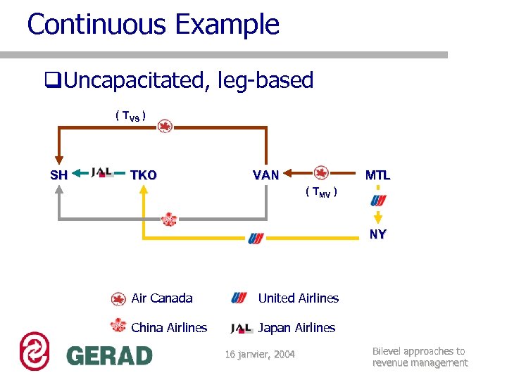
Continuous Example q. Uncapacitated, leg-based ( TVS ) SH TKO VAN MTL ( TMV ) NY Air Canada United Airlines China Airlines Japan Airlines 16 janvier, 2004 Bilevel approaches to revenue management
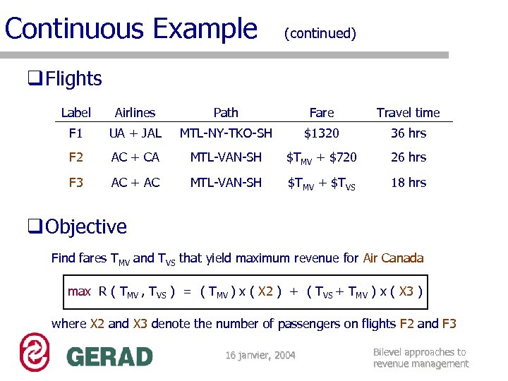
Continuous Example (continued) q Flights Label Airlines Path Fare Travel time F 1 UA + JAL MTL-NY-TKO-SH $1320 36 hrs F 2 AC + CA MTL-VAN-SH $TMV + $720 26 hrs F 3 AC + AC MTL-VAN-SH $TMV + $TVS 18 hrs q Objective Find fares TMV and TVS that yield maximum revenue for Air Canada max R ( TMV , TVS ) = ( TMV ) x ( X 2 ) + ( TVS + TMV ) x ( X 3 ) where X 2 and X 3 denote the number of passengers on flights F 2 and F 3 16 janvier, 2004 Bilevel approaches to revenue management
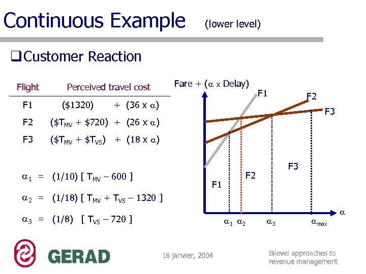
Continuous Example (lower level) q Customer Reaction Flight F 1 Fare + ( Perceived travel cost ($1320) x Delay) F 1 F 2 + (36 x ) F 2 ($TMV + $720) + (26 x ) F 3 ($TMV + $TVS) + (18 x ) 1 = (1/10) [ TMV – 600 ] F 3 F 2 F 1 2 = (1/18) [ TMV + TVS – 1320 ] 3 = (1/8) [ TVS – 720 ] 1 2 16 janvier, 2004 3 max Bilevel approaches to revenue management
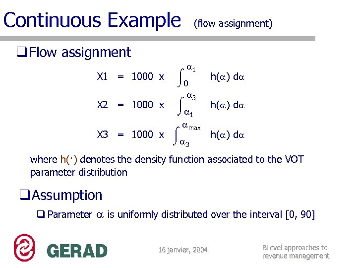
Continuous Example q Flow assignment (flow assignment) 1 0 3 X 2 = 1000 x 1 max X 3 = 1000 x 3 X 1 = 1000 x h( ) d where h(·) denotes the density function associated to the VOT parameter distribution q Assumption q Parameter is uniformly distributed over the interval [0, 90] 16 janvier, 2004 Bilevel approaches to revenue management
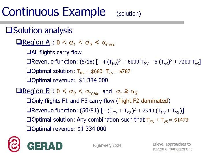
Continuous Example (solution) q Solution analysis q. Region A : 0 < 1 < 3 < max q. All flights carry flow q. Revenue function: (5/18) [– 4 (TMV)2 + 6000 TMV – 5 (TVS)2 + 7200 TVS] q. Optimal solution: TMV = $683 TVS = $787 q. Optimal revenue: $1 334 000 q. Region B : 0 < 2 < max and 1 3 q. Only flights F 1 and F 3 carry flow (flight F 2 dominated) q. Revenue function: (50/81) [– (TMV + TVS )2 + 2940 (TMV + TVS )] q. Optimal solution: Any combination such that TMV + TVS = $1470 q. Optimal revenue: $1 334 000 16 janvier, 2004 Bilevel approaches to revenue management
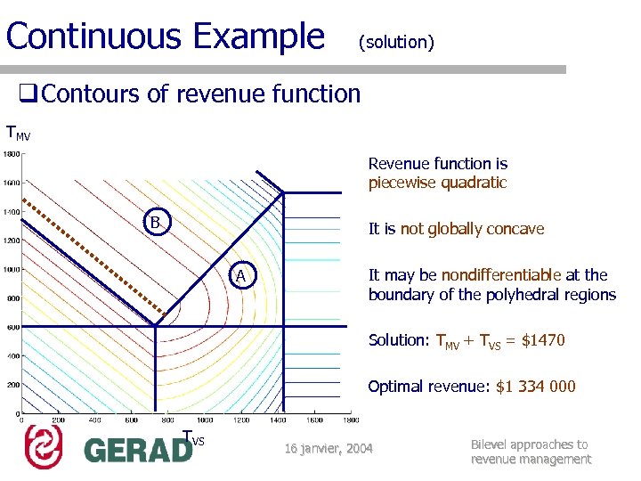
Continuous Example (solution) q Contours of revenue function TMV q Revenue function is piecewise quadratic B q It is not globally concave A q It may be nondifferentiable at the boundary of the polyhedral regions q Solution: TMV + TVS = $1470 q Optimal revenue: $1 334 000 TVS 16 janvier, 2004 Bilevel approaches to revenue management
f2b58823729919b0e6291c30b3b8a19d.ppt