4303a300952882371519e116d7e110e8.ppt
- Количество слайдов: 134
Bellwether Analysis Data Mining (with many slides due to Gehrke, Garofalakis, Rastogi) Raghu Ramakrishnan Yahoo! Research University of Wisconsin–Madison (on leave) TECS 2007 R. Ramakrishnan, Yahoo! Research
Introduction TECS 2007, Data Mining R. Bee-Chung Chen, Raghu Ramakrishnan, Jude Shavlik, Pradeep Tamma Ramakrishnan, Yahoo! Research 2
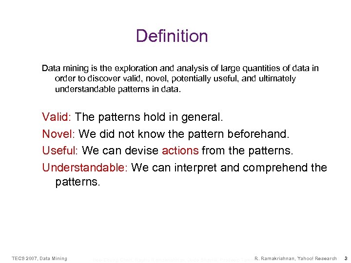
Definition Data mining is the exploration and analysis of large quantities of data in order to discover valid, novel, potentially useful, and ultimately understandable patterns in data. Valid: The patterns hold in general. Novel: We did not know the pattern beforehand. Useful: We can devise actions from the patterns. Understandable: We can interpret and comprehend the patterns. TECS 2007, Data Mining R. Bee-Chung Chen, Raghu Ramakrishnan, Jude Shavlik, Pradeep Tamma Ramakrishnan, Yahoo! Research 3
Case Study: Bank • Business goal: Sell more home equity loans • Current models: – Customers with college-age children use home equity loans to pay for tuition – Customers with variable income use home equity loans to even out stream of income • Data: – Large data warehouse – Consolidates data from 42 operational data sources TECS 2007, Data Mining R. Bee-Chung Chen, Raghu Ramakrishnan, Jude Shavlik, Pradeep Tamma Ramakrishnan, Yahoo! Research 4
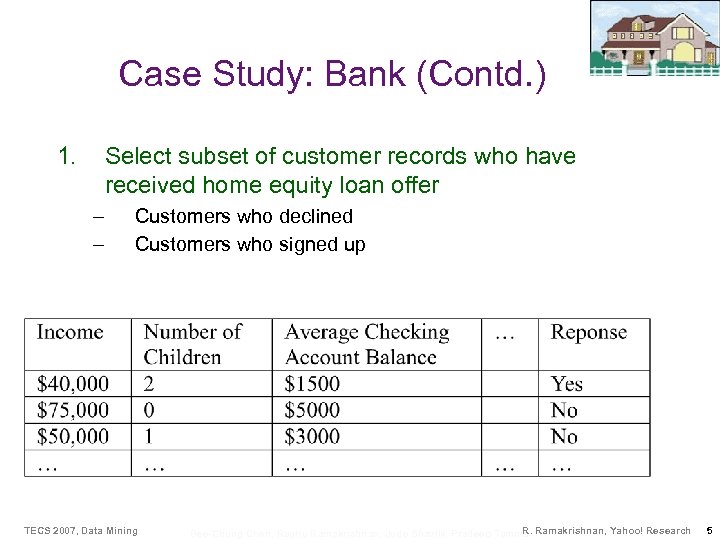
Case Study: Bank (Contd. ) 1. Select subset of customer records who have received home equity loan offer – – Customers who declined Customers who signed up TECS 2007, Data Mining R. Bee-Chung Chen, Raghu Ramakrishnan, Jude Shavlik, Pradeep Tamma Ramakrishnan, Yahoo! Research 5
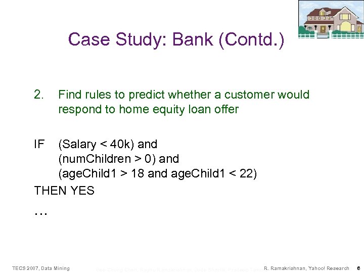
Case Study: Bank (Contd. ) 2. Find rules to predict whether a customer would respond to home equity loan offer IF (Salary < 40 k) and (num. Children > 0) and (age. Child 1 > 18 and age. Child 1 < 22) THEN YES … TECS 2007, Data Mining R. Bee-Chung Chen, Raghu Ramakrishnan, Jude Shavlik, Pradeep Tamma Ramakrishnan, Yahoo! Research 6
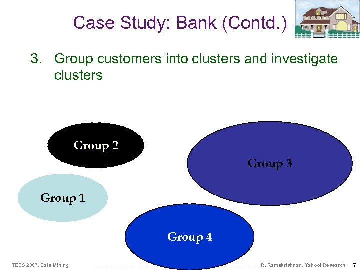
Case Study: Bank (Contd. ) 3. Group customers into clusters and investigate clusters Group 2 Group 3 Group 1 Group 4 TECS 2007, Data Mining R. Bee-Chung Chen, Raghu Ramakrishnan, Jude Shavlik, Pradeep Tamma Ramakrishnan, Yahoo! Research 7
Case Study: Bank (Contd. ) 4. Evaluate results: – – TECS 2007, Data Mining Many “uninteresting” clusters One interesting cluster! Customers with both business and personal accounts; unusually high percentage of likely respondents R. Bee-Chung Chen, Raghu Ramakrishnan, Jude Shavlik, Pradeep Tamma Ramakrishnan, Yahoo! Research 8
Example: Bank (Contd. ) Action: • New marketing campaign Result: • Acceptance rate for home equity offers more than doubled TECS 2007, Data Mining R. Bee-Chung Chen, Raghu Ramakrishnan, Jude Shavlik, Pradeep Tamma Ramakrishnan, Yahoo! Research 9
Example Application: Fraud Detection • Industries: Health care, retail, credit card services, telecom, B 2 B relationships • Approach: – Use historical data to build models of fraudulent behavior – Deploy models to identify fraudulent instances TECS 2007, Data Mining R. Bee-Chung Chen, Raghu Ramakrishnan, Jude Shavlik, Pradeep Tamma Ramakrishnan, Yahoo! Research 10
Fraud Detection (Contd. ) • Examples: – Auto insurance: Detect groups of people who stage accidents to collect insurance – Medical insurance: Fraudulent claims – Money laundering: Detect suspicious money transactions (US Treasury's Financial Crimes Enforcement Network) – Telecom industry: Find calling patterns that deviate from a norm (origin and destination of the call, duration, time of day, day of week). TECS 2007, Data Mining R. Bee-Chung Chen, Raghu Ramakrishnan, Jude Shavlik, Pradeep Tamma Ramakrishnan, Yahoo! Research 11
Other Example Applications • • CPG: Promotion analysis Retail: Category management Telecom: Call usage analysis, churn Healthcare: Claims analysis, fraud detection Transportation/Distribution: Logistics management Financial Services: Credit analysis, fraud detection Data service providers: Value-added data analysis TECS 2007, Data Mining R. Bee-Chung Chen, Raghu Ramakrishnan, Jude Shavlik, Pradeep Tamma Ramakrishnan, Yahoo! Research 12
What is a Data Mining Model? A data mining model is a description of a certain aspect of a dataset. It produces output values for an assigned set of inputs. Examples: • Clustering • Linear regression model • Classification model • Frequent itemsets and association rules • Support Vector Machines TECS 2007, Data Mining R. Bee-Chung Chen, Raghu Ramakrishnan, Jude Shavlik, Pradeep Tamma Ramakrishnan, Yahoo! Research 13
Data Mining Methods TECS 2007, Data Mining R. Bee-Chung Chen, Raghu Ramakrishnan, Jude Shavlik, Pradeep Tamma Ramakrishnan, Yahoo! Research 14
Overview • Several well-studied tasks – Classification – Clustering – Frequent Patterns • Many methods proposed for each • Focus in database and data mining community: – Scalability – Managing the process – Exploratory analysis TECS 2007, Data Mining R. Bee-Chung Chen, Raghu Ramakrishnan, Jude Shavlik, Pradeep Tamma Ramakrishnan, Yahoo! Research 15
Classification Goal: Learn a function that assigns a record to one of several predefined classes. Requirements on the model: High accuracy – Understandable by humans, interpretable – Fast construction for very large training databases – TECS 2007, Data Mining R. Bee-Chung Chen, Raghu Ramakrishnan, Jude Shavlik, Pradeep Tamma Ramakrishnan, Yahoo! Research
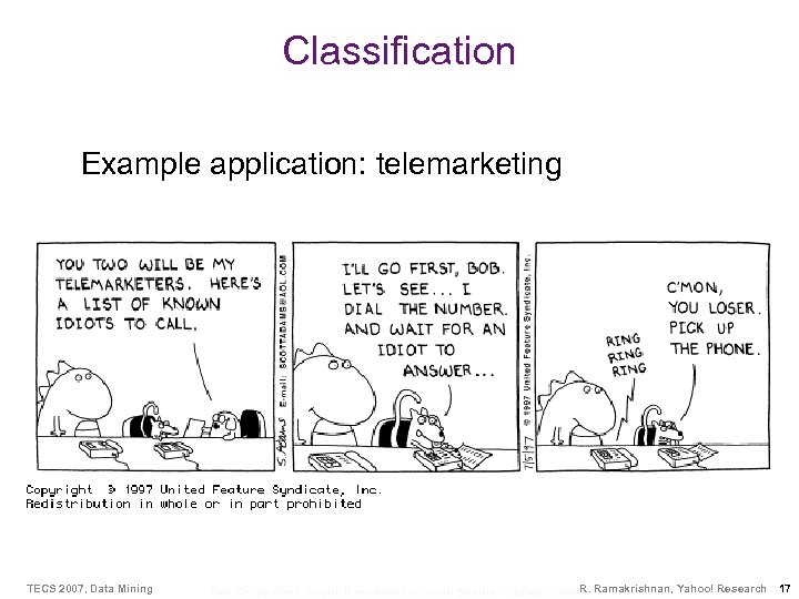
Classification Example application: telemarketing TECS 2007, Data Mining R. Bee-Chung Chen, Raghu Ramakrishnan, Jude Shavlik, Pradeep Tamma Ramakrishnan, Yahoo! Research 17
Classification (Contd. ) Decision trees are one approach to classification. • Other approaches include: • – – – Linear Discriminant Analysis k-nearest neighbor methods Logistic regression Neural networks Support Vector Machines TECS 2007, Data Mining R. Bee-Chung Chen, Raghu Ramakrishnan, Jude Shavlik, Pradeep Tamma Ramakrishnan, Yahoo! Research
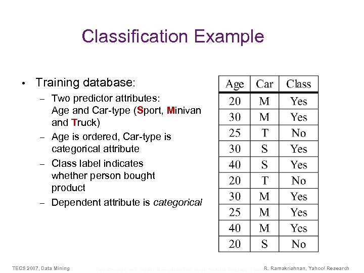
Classification Example • Training database: Two predictor attributes: Age and Car-type (Sport, Minivan and Truck) – Age is ordered, Car-type is categorical attribute – Class label indicates whether person bought product – Dependent attribute is categorical – TECS 2007, Data Mining R. Bee-Chung Chen, Raghu Ramakrishnan, Jude Shavlik, Pradeep Tamma Ramakrishnan, Yahoo! Research
Classification Problem • If Y is categorical, the problem is a classification problem, and we use C instead of Y. |dom(C)| = J, the number of classes. • C is the class label, d is called a classifier. • Let r be a record randomly drawn from P. Define the misclassification rate of d: RT(d, P) = P(d(r. X 1, …, r. Xk) != r. C) • Problem definition: Given dataset D that is a random sample from probability distribution P, find classifier d such that RT(d, P) is minimized. TECS 2007, Data Mining R. Bee-Chung Chen, Raghu Ramakrishnan, Jude Shavlik, Pradeep Tamma Ramakrishnan, Yahoo! Research 22
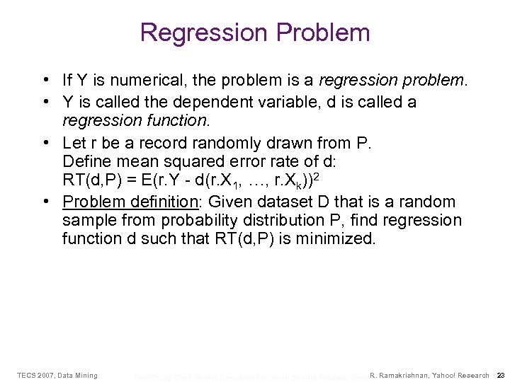
Regression Problem • If Y is numerical, the problem is a regression problem. • Y is called the dependent variable, d is called a regression function. • Let r be a record randomly drawn from P. Define mean squared error rate of d: RT(d, P) = E(r. Y - d(r. X 1, …, r. Xk))2 • Problem definition: Given dataset D that is a random sample from probability distribution P, find regression function d such that RT(d, P) is minimized. TECS 2007, Data Mining R. Bee-Chung Chen, Raghu Ramakrishnan, Jude Shavlik, Pradeep Tamma Ramakrishnan, Yahoo! Research 23
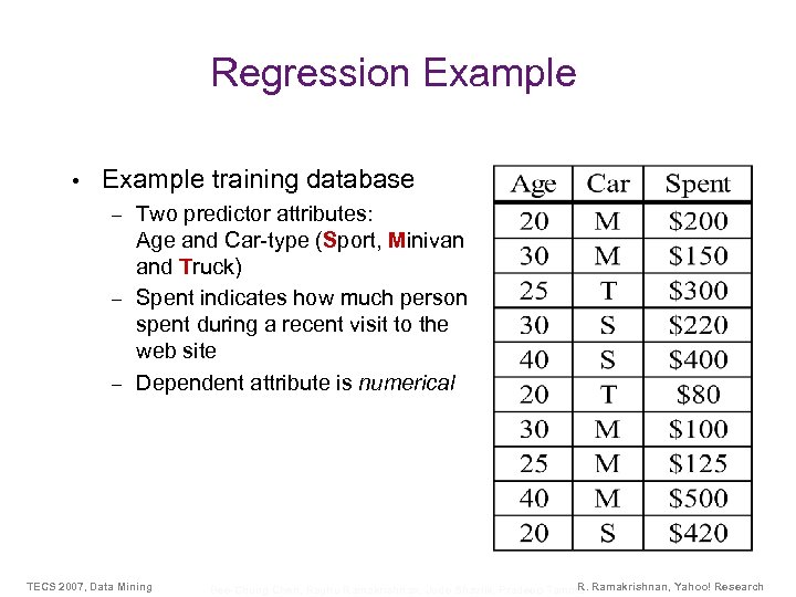
Regression Example • Example training database Two predictor attributes: Age and Car-type (Sport, Minivan and Truck) – Spent indicates how much person spent during a recent visit to the web site – Dependent attribute is numerical – TECS 2007, Data Mining R. Bee-Chung Chen, Raghu Ramakrishnan, Jude Shavlik, Pradeep Tamma Ramakrishnan, Yahoo! Research
Decision Trees TECS 2007, Data Mining R. Bee-Chung Chen, Raghu Ramakrishnan, Jude Shavlik, Pradeep Tamma Ramakrishnan, Yahoo! Research 25
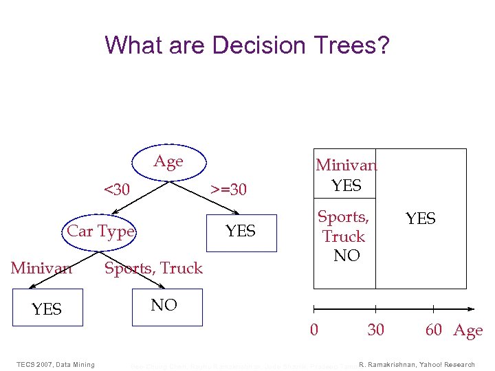
What are Decision Trees? Age <30 >=30 YES Car Type Minivan YES Sports, Truck NO NO 0 TECS 2007, Data Mining YES 30 60 Age R. Bee-Chung Chen, Raghu Ramakrishnan, Jude Shavlik, Pradeep Tamma Ramakrishnan, Yahoo! Research
Decision Trees • A decision tree T encodes d (a classifier or regression function) in form of a tree. • A node t in T without children is called a leaf node. Otherwise t is called an internal node. TECS 2007, Data Mining R. Bee-Chung Chen, Raghu Ramakrishnan, Jude Shavlik, Pradeep Tamma Ramakrishnan, Yahoo! Research 27
Internal Nodes • Each internal node has an associated splitting predicate. Most common are binary predicates. Example predicates: – Age <= 20 – Profession in {student, teacher} – 5000*Age + 3*Salary – 10000 > 0 TECS 2007, Data Mining R. Bee-Chung Chen, Raghu Ramakrishnan, Jude Shavlik, Pradeep Tamma Ramakrishnan, Yahoo! Research 28
Leaf Nodes Consider leaf node t: • Classification problem: Node t is labeled with one class label c in dom(C) • Regression problem: Two choices – Piecewise constant model: t is labeled with a constant y in dom(Y). – Piecewise linear model: t is labeled with a linear model Y = yt + Σ ai. Xi TECS 2007, Data Mining R. Bee-Chung Chen, Raghu Ramakrishnan, Jude Shavlik, Pradeep Tamma Ramakrishnan, Yahoo! Research 30
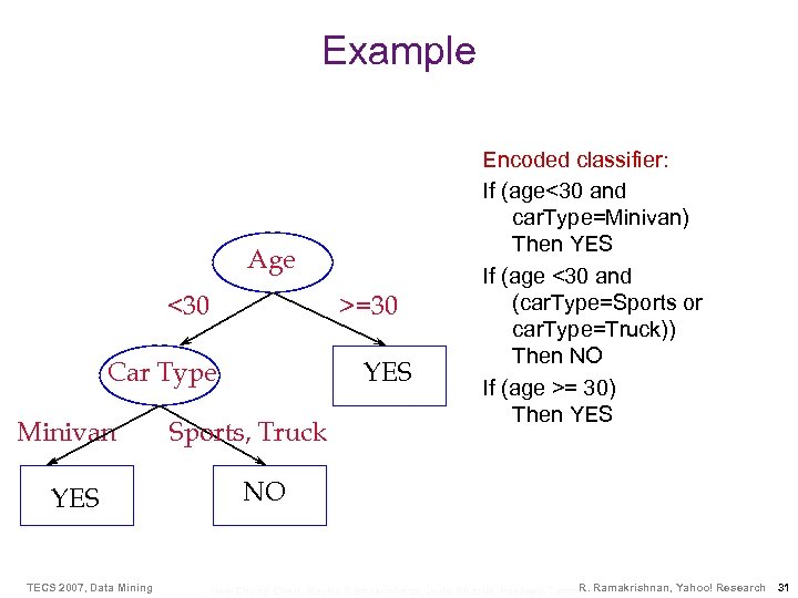
Example Age <30 >=30 YES Car Type Minivan YES TECS 2007, Data Mining Sports, Truck Encoded classifier: If (age<30 and car. Type=Minivan) Then YES If (age <30 and (car. Type=Sports or car. Type=Truck)) Then NO If (age >= 30) Then YES NO R. Bee-Chung Chen, Raghu Ramakrishnan, Jude Shavlik, Pradeep Tamma Ramakrishnan, Yahoo! Research 31
Issues in Tree Construction • Three algorithmic components: Split Selection Method – Pruning Method – Data Access Method – TECS 2007, Data Mining R. Bee-Chung Chen, Raghu Ramakrishnan, Jude Shavlik, Pradeep Tamma Ramakrishnan, Yahoo! Research
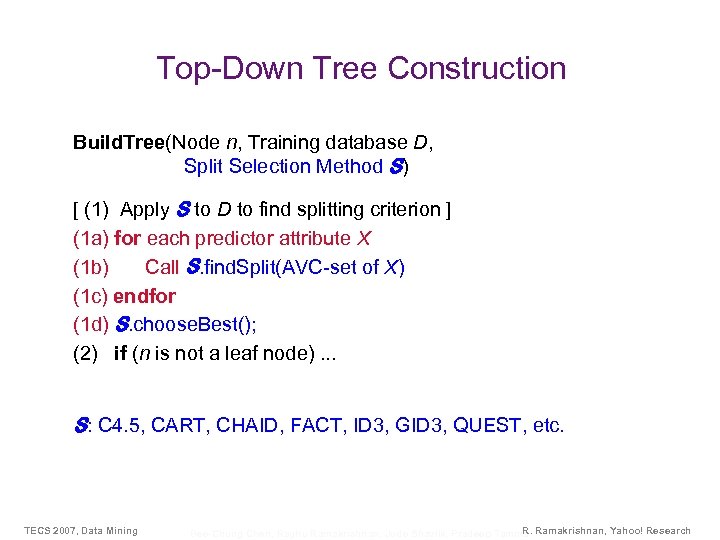
Top-Down Tree Construction Build. Tree(Node n, Training database D, Split Selection Method S) [ (1) Apply S to D to find splitting criterion ] (1 a) for each predictor attribute X (1 b) Call S. find. Split(AVC-set of X) (1 c) endfor (1 d) S. choose. Best(); (2) if (n is not a leaf node). . . S: C 4. 5, CART, CHAID, FACT, ID 3, GID 3, QUEST, etc. TECS 2007, Data Mining R. Bee-Chung Chen, Raghu Ramakrishnan, Jude Shavlik, Pradeep Tamma Ramakrishnan, Yahoo! Research
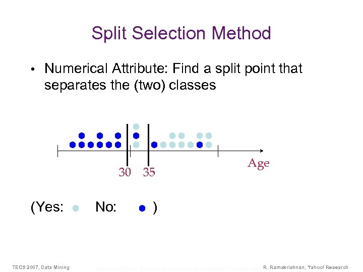
Split Selection Method • Numerical Attribute: Find a split point that separates the (two) classes 30 (Yes: TECS 2007, Data Mining No: 35 Age ) R. Bee-Chung Chen, Raghu Ramakrishnan, Jude Shavlik, Pradeep Tamma Ramakrishnan, Yahoo! Research
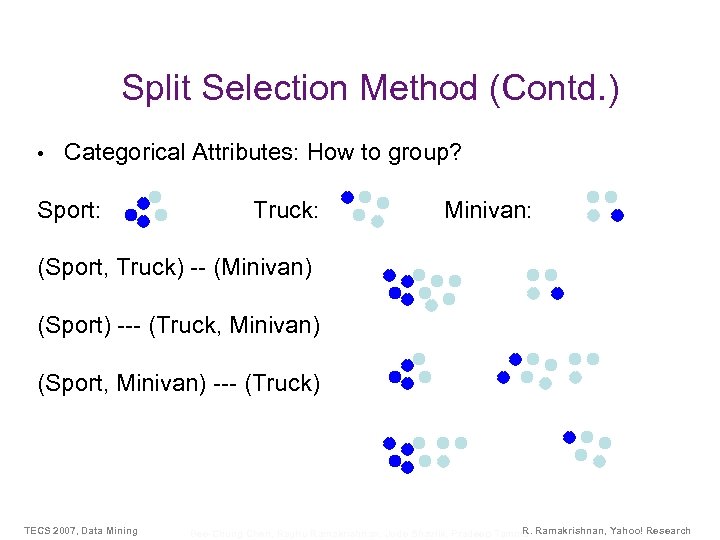
Split Selection Method (Contd. ) • Categorical Attributes: How to group? Sport: Truck: Minivan: (Sport, Truck) -- (Minivan) (Sport) --- (Truck, Minivan) (Sport, Minivan) --- (Truck) TECS 2007, Data Mining R. Bee-Chung Chen, Raghu Ramakrishnan, Jude Shavlik, Pradeep Tamma Ramakrishnan, Yahoo! Research
Impurity-based Split Selection Methods • Split selection method has two parts: Search space of possible splitting criteria. Example: All splits of the form “age <= c”. – Quality assessment of a splitting criterion – Need to quantify the quality of a split: Impurity function • Example impurity functions: Entropy, gini-index, chi-square index • TECS 2007, Data Mining R. Bee-Chung Chen, Raghu Ramakrishnan, Jude Shavlik, Pradeep Tamma Ramakrishnan, Yahoo! Research
Data Access Method • Goal: Scalable decision tree construction, using the complete training database TECS 2007, Data Mining R. Bee-Chung Chen, Raghu Ramakrishnan, Jude Shavlik, Pradeep Tamma Ramakrishnan, Yahoo! Research
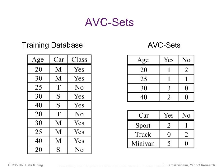
AVC-Sets Training Database TECS 2007, Data Mining AVC-Sets R. Bee-Chung Chen, Raghu Ramakrishnan, Jude Shavlik, Pradeep Tamma Ramakrishnan, Yahoo! Research
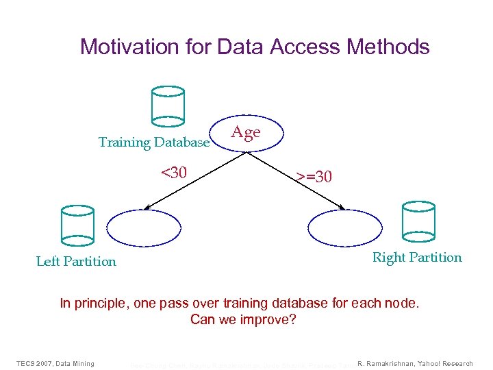
Motivation for Data Access Methods Training Database <30 Left Partition Age >=30 Right Partition In principle, one pass over training database for each node. Can we improve? TECS 2007, Data Mining R. Bee-Chung Chen, Raghu Ramakrishnan, Jude Shavlik, Pradeep Tamma Ramakrishnan, Yahoo! Research
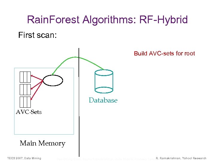
Rain. Forest Algorithms: RF-Hybrid First scan: Build AVC-sets for root Database AVC-Sets Main Memory TECS 2007, Data Mining R. Bee-Chung Chen, Raghu Ramakrishnan, Jude Shavlik, Pradeep Tamma Ramakrishnan, Yahoo! Research
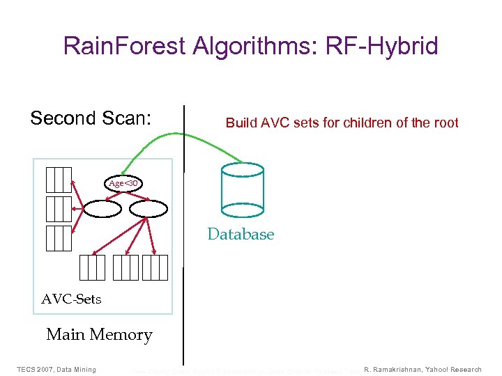
Rain. Forest Algorithms: RF-Hybrid Second Scan: Build AVC sets for children of the root Age<30 Database AVC-Sets Main Memory TECS 2007, Data Mining R. Bee-Chung Chen, Raghu Ramakrishnan, Jude Shavlik, Pradeep Tamma Ramakrishnan, Yahoo! Research
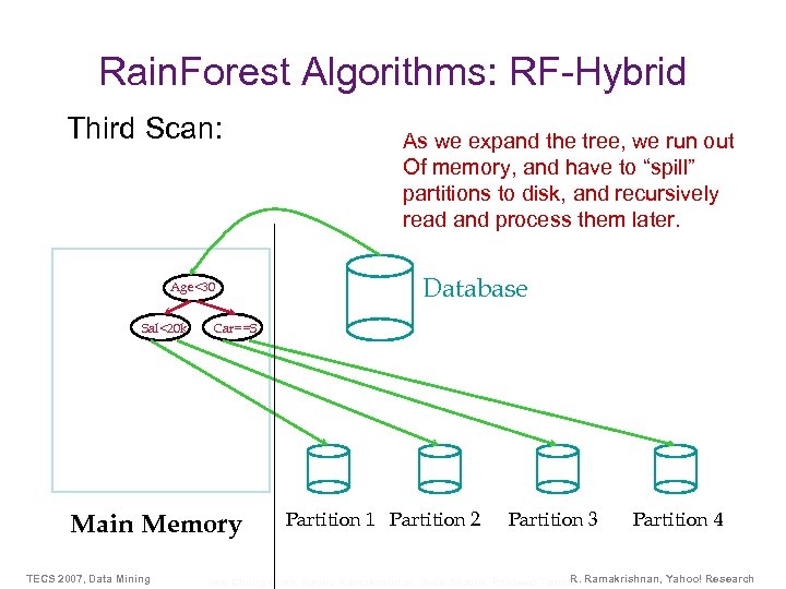
Rain. Forest Algorithms: RF-Hybrid Third Scan: Age<30 Sal<20 k Database Car==S Main Memory TECS 2007, Data Mining As we expand the tree, we run out Of memory, and have to “spill” partitions to disk, and recursively read and process them later. Partition 1 Partition 2 Partition 3 Partition 4 R. Bee-Chung Chen, Raghu Ramakrishnan, Jude Shavlik, Pradeep Tamma Ramakrishnan, Yahoo! Research
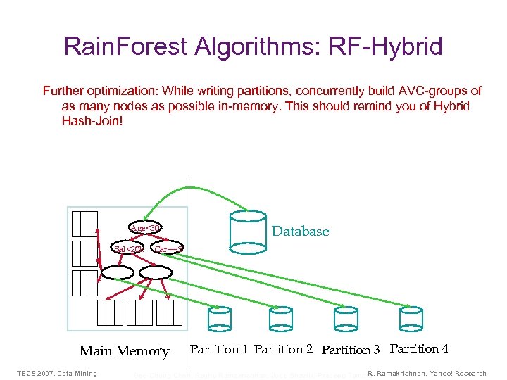
Rain. Forest Algorithms: RF-Hybrid Further optimization: While writing partitions, concurrently build AVC-groups of as many nodes as possible in-memory. This should remind you of Hybrid Hash-Join! Age<30 Sal<20 k Car==S Main Memory TECS 2007, Data Mining Database Partition 1 Partition 2 Partition 3 Partition 4 R. Bee-Chung Chen, Raghu Ramakrishnan, Jude Shavlik, Pradeep Tamma Ramakrishnan, Yahoo! Research
CLUSTERING TECS 2007, Data Mining R. Bee-Chung Chen, Raghu Ramakrishnan, Jude Shavlik, Pradeep Tamma Ramakrishnan, Yahoo! Research 44
Problem • Given points in a multidimensional space, group them into a small number of clusters, using some measure of “nearness” – E. g. , Cluster documents by topic – E. g. , Cluster users by similar interests TECS 2007, Data Mining R. Bee-Chung Chen, Raghu Ramakrishnan, Jude Shavlik, Pradeep Tamma Ramakrishnan, Yahoo! Research 45
Clustering • Output: (k) groups of records called clusters, such that the records within a group are more similar to records in other groups – Representative points for each cluster – Labeling of each record with each cluster number – Other description of each cluster • This is unsupervised learning: No record labels are given to learn from • Usage: – Exploratory data mining – Preprocessing step (e. g. , outlier detection) TECS 2007, Data Mining R. Bee-Chung Chen, Raghu Ramakrishnan, Jude Shavlik, Pradeep Tamma Ramakrishnan, Yahoo! Research 46
Clustering (Contd. ) • Requirements: Need to define “similarity” between records • Important: Use the “right” similarity (distance) function – Scale or normalize all attributes. Example: seconds, hours, days – Assign different weights to reflect importance of the attribute – Choose appropriate measure (e. g. , L 1, L 2) TECS 2007, Data Mining R. Bee-Chung Chen, Raghu Ramakrishnan, Jude Shavlik, Pradeep Tamma Ramakrishnan, Yahoo! Research 49
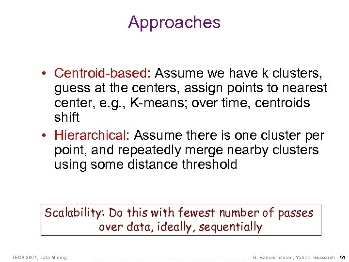
Approaches • Centroid-based: Assume we have k clusters, guess at the centers, assign points to nearest center, e. g. , K-means; over time, centroids shift • Hierarchical: Assume there is one cluster point, and repeatedly merge nearby clusters using some distance threshold Scalability: Do this with fewest number of passes over data, ideally, sequentially TECS 2007, Data Mining R. Bee-Chung Chen, Raghu Ramakrishnan, Jude Shavlik, Pradeep Tamma Ramakrishnan, Yahoo! Research 51
Scalable Clustering Algorithms for Numeric Attributes CLARANS DBSCAN BIRCH CLIQUE CURE ……. • Above algorithms can be used to cluster documents after reducing their dimensionality using SVD TECS 2007, Data Mining R. Bee-Chung Chen, Raghu Ramakrishnan, Jude Shavlik, Pradeep Tamma Ramakrishnan, Yahoo! Research 54
![Birch [ZRL 96] Pre-cluster data points using “CF-tree” data structure TECS 2007, Data Mining Birch [ZRL 96] Pre-cluster data points using “CF-tree” data structure TECS 2007, Data Mining](https://present5.com/presentation/4303a300952882371519e116d7e110e8/image-47.jpg)
Birch [ZRL 96] Pre-cluster data points using “CF-tree” data structure TECS 2007, Data Mining R. Bee-Chung Chen, Raghu Ramakrishnan, Jude Shavlik, Pradeep Tamma Ramakrishnan, Yahoo! Research
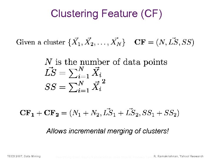
Clustering Feature (CF) Allows incremental merging of clusters! TECS 2007, Data Mining R. Bee-Chung Chen, Raghu Ramakrishnan, Jude Shavlik, Pradeep Tamma Ramakrishnan, Yahoo! Research
Points to Note • Basic algorithm works in a single pass to condense metric data using spherical summaries – Can be incremental • Additional passes cluster CFs to detect nonspherical clusters • Approximates density function • Extensions to non-metric data TECS 2007, Data Mining R. Bee-Chung Chen, Raghu Ramakrishnan, Jude Shavlik, Pradeep Tamma Ramakrishnan, Yahoo! Research 60
Market Basket Analysis: Frequent Itemsets TECS 2007, Data Mining R. Bee-Chung Chen, Raghu Ramakrishnan, Jude Shavlik, Pradeep Tamma Ramakrishnan, Yahoo! Research 63
Market Basket Analysis • Consider shopping cart filled with several items • Market basket analysis tries to answer the following questions: – Who makes purchases – What do customers buy TECS 2007, Data Mining R. Bee-Chung Chen, Raghu Ramakrishnan, Jude Shavlik, Pradeep Tamma Ramakrishnan, Yahoo! Research 64
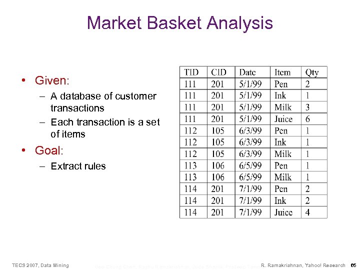
Market Basket Analysis • Given: – A database of customer transactions – Each transaction is a set of items • Goal: – Extract rules TECS 2007, Data Mining R. Bee-Chung Chen, Raghu Ramakrishnan, Jude Shavlik, Pradeep Tamma Ramakrishnan, Yahoo! Research 65
Market Basket Analysis (Contd. ) • Co-occurrences – 80% of all customers purchase items X, Y and Z together. • Association rules – 60% of all customers who purchase X and Y also buy Z. • Sequential patterns – 60% of customers who first buy X also purchase Y within three weeks. TECS 2007, Data Mining R. Bee-Chung Chen, Raghu Ramakrishnan, Jude Shavlik, Pradeep Tamma Ramakrishnan, Yahoo! Research 66
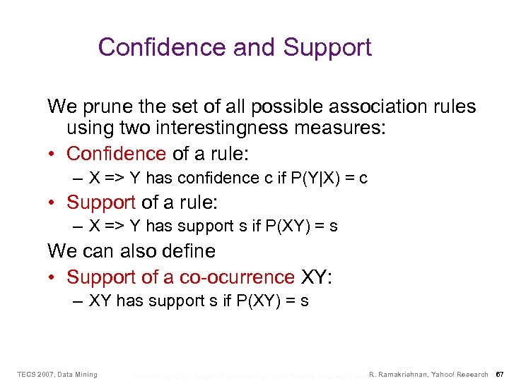
Confidence and Support We prune the set of all possible association rules using two interestingness measures: • Confidence of a rule: – X => Y has confidence c if P(Y|X) = c • Support of a rule: – X => Y has support s if P(XY) = s We can also define • Support of a co-ocurrence XY: – XY has support s if P(XY) = s TECS 2007, Data Mining R. Bee-Chung Chen, Raghu Ramakrishnan, Jude Shavlik, Pradeep Tamma Ramakrishnan, Yahoo! Research 67
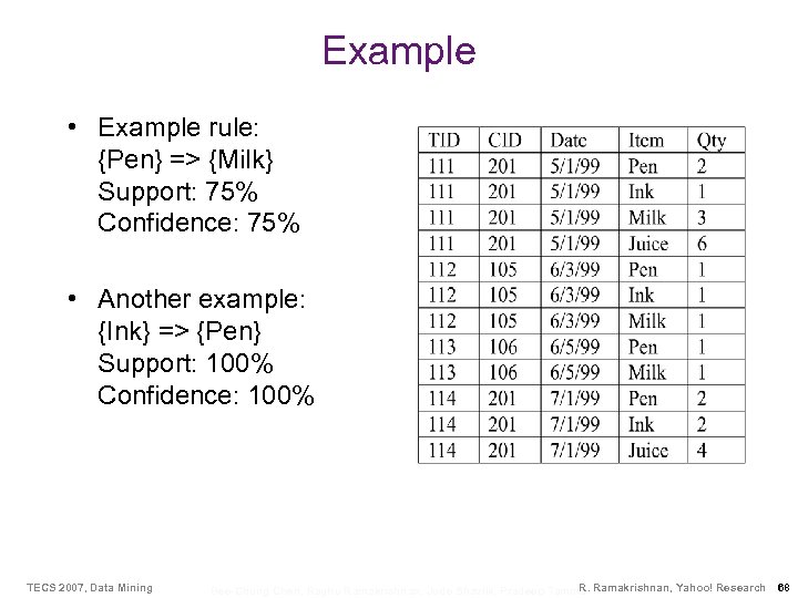
Example • Example rule: {Pen} => {Milk} Support: 75% Confidence: 75% • Another example: {Ink} => {Pen} Support: 100% Confidence: 100% TECS 2007, Data Mining R. Bee-Chung Chen, Raghu Ramakrishnan, Jude Shavlik, Pradeep Tamma Ramakrishnan, Yahoo! Research 68
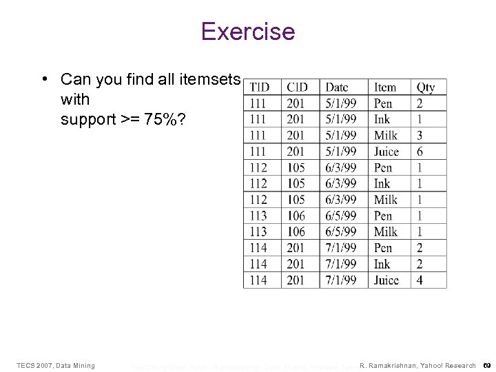
Exercise • Can you find all itemsets with support >= 75%? TECS 2007, Data Mining R. Bee-Chung Chen, Raghu Ramakrishnan, Jude Shavlik, Pradeep Tamma Ramakrishnan, Yahoo! Research 69
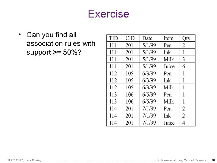
Exercise • Can you find all association rules with support >= 50%? TECS 2007, Data Mining R. Bee-Chung Chen, Raghu Ramakrishnan, Jude Shavlik, Pradeep Tamma Ramakrishnan, Yahoo! Research 70
Extensions • Imposing constraints – – – TECS 2007, Data Mining Only find rules involving the dairy department Only find rules involving expensive products Only find rules with “whiskey” on the right hand side Only find rules with “milk” on the left hand side Hierarchies on the items Calendars (every Sunday, every 1 st of the month) R. Bee-Chung Chen, Raghu Ramakrishnan, Jude Shavlik, Pradeep Tamma Ramakrishnan, Yahoo! Research 71
Market Basket Analysis: Applications • Sample Applications – – – TECS 2007, Data Mining Direct marketing Fraud detection for medical insurance Floor/shelf planning Web site layout Cross-selling R. Bee-Chung Chen, Raghu Ramakrishnan, Jude Shavlik, Pradeep Tamma Ramakrishnan, Yahoo! Research 72
DBMS Support for DM TECS 2007, Data Mining R. Bee-Chung Chen, Raghu Ramakrishnan, Jude Shavlik, Pradeep Tamma Ramakrishnan, Yahoo! Research 73
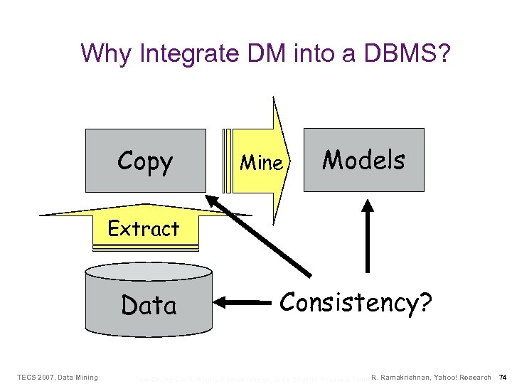
Why Integrate DM into a DBMS? Copy Mine Models Extract Data TECS 2007, Data Mining Consistency? R. Bee-Chung Chen, Raghu Ramakrishnan, Jude Shavlik, Pradeep Tamma Ramakrishnan, Yahoo! Research 74
Integration Objectives • Avoid isolation of querying from mining – Difficult to do “ad-hoc” mining • Provide simple programming approach to creating and using DM models Analysts (users) TECS 2007, Data Mining • Make it possible to add new models • Make it possible to add new, scalable algorithms DM Vendors R. Bee-Chung Chen, Raghu Ramakrishnan, Jude Shavlik, Pradeep Tamma Ramakrishnan, Yahoo! Research 75
SQL/MM: Data Mining • A collection of classes that provide a standard interface for invoking DM algorithms from SQL systems. • Four data models are supported: – – Frequent itemsets, association rules Clusters Regression trees Classification trees TECS 2007, Data Mining R. Bee-Chung Chen, Raghu Ramakrishnan, Jude Shavlik, Pradeep Tamma Ramakrishnan, Yahoo! Research 76
DATA MINING SUPPORT IN MICROSOFT SQL SERVER * * Thanks to Surajit Chaudhuri for permission to use/adapt his slides TECS 2007, Data Mining R. Bee-Chung Chen, Raghu Ramakrishnan, Jude Shavlik, Pradeep Tamma Ramakrishnan, Yahoo! Research 77
Key Design Decisions • Adopt relational data representation – A Data Mining Model (DMM) as a “tabular” object (externally; can be represented differently internally) • Language-based interface – Extension of SQL – Standard syntax TECS 2007, Data Mining R. Bee-Chung Chen, Raghu Ramakrishnan, Jude Shavlik, Pradeep Tamma Ramakrishnan, Yahoo! Research 78
DM Concepts to Support • • Representation of input (cases) Representation of models Specification of training step Specification of prediction step Should be independent of specific algorithms TECS 2007, Data Mining R. Bee-Chung Chen, Raghu Ramakrishnan, Jude Shavlik, Pradeep Tamma Ramakrishnan, Yahoo! Research 79
What are “Cases”? • DM algorithms analyze “cases” • The “case” is the entity being categorized and classified • Examples – Customer credit risk analysis: Case = Customer – Product profitability analysis: Case = Product – Promotion success analysis: Case = Promotion • Each case encapsulates all we know about the entity TECS 2007, Data Mining R. Bee-Chung Chen, Raghu Ramakrishnan, Jude Shavlik, Pradeep Tamma Ramakrishnan, Yahoo! Research 80
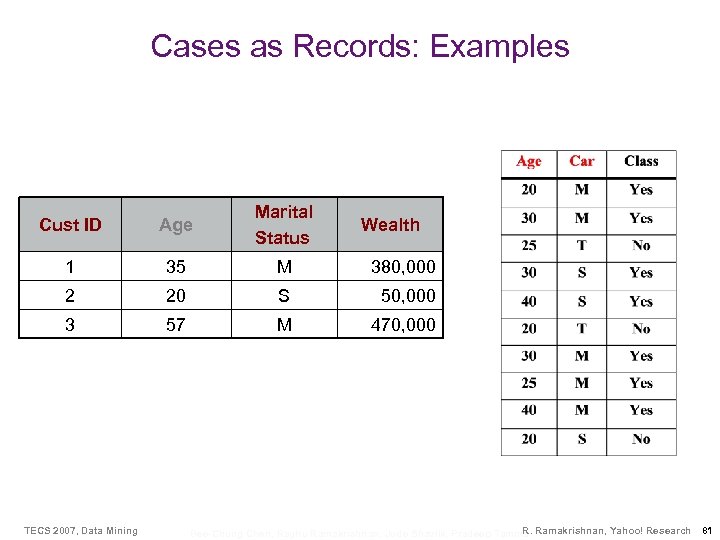
Cases as Records: Examples Cust ID Age Marital Status 1 35 M 380, 000 2 20 S 50, 000 3 57 M 470, 000 TECS 2007, Data Mining Wealth R. Bee-Chung Chen, Raghu Ramakrishnan, Jude Shavlik, Pradeep Tamma Ramakrishnan, Yahoo! Research 81
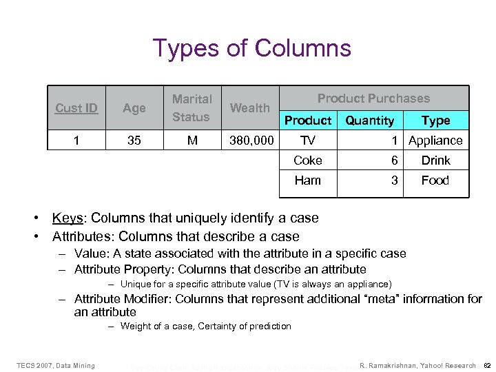
Types of Columns Cust ID Age Marital Status Wealth 1 35 M Product Purchases 380, 000 Product TV Quantity Type 1 Appliance Coke 6 Drink Ham 3 Food • Keys: Columns that uniquely identify a case • Attributes: Columns that describe a case – Value: A state associated with the attribute in a specific case – Attribute Property: Columns that describe an attribute – Unique for a specific attribute value (TV is always an appliance) – Attribute Modifier: Columns that represent additional “meta” information for an attribute – Weight of a case, Certainty of prediction TECS 2007, Data Mining R. Bee-Chung Chen, Raghu Ramakrishnan, Jude Shavlik, Pradeep Tamma Ramakrishnan, Yahoo! Research 82
More on Columns • Properties describe attributes – Can represent generalization hierarchy • Distribution information associated with attributes – Discrete/Continuous – Nature of Continuous distributions • Normal, Log_Normal – Other Properties (e. g. , ordered, not null) TECS 2007, Data Mining R. Bee-Chung Chen, Raghu Ramakrishnan, Jude Shavlik, Pradeep Tamma Ramakrishnan, Yahoo! Research 83
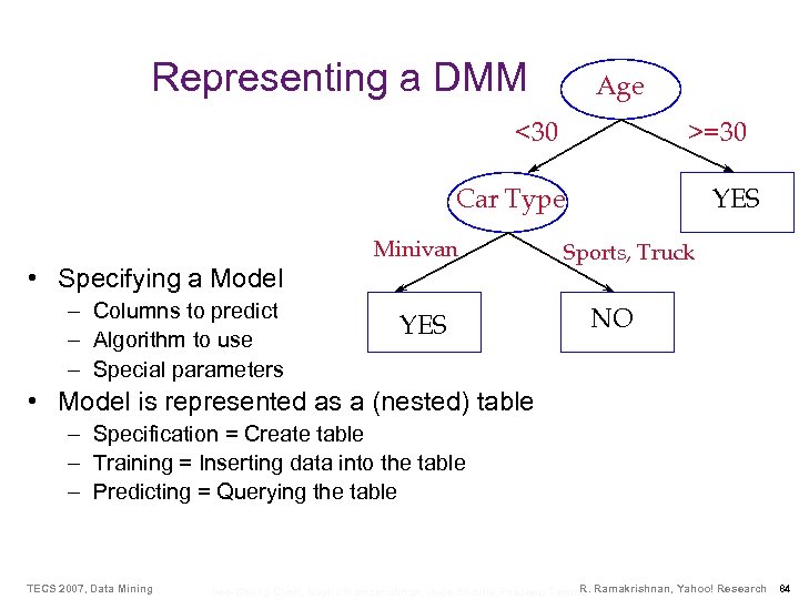
Representing a DMM Age <30 >=30 YES Car Type Minivan • Specifying a Model – Columns to predict – Algorithm to use – Special parameters YES Sports, Truck NO • Model is represented as a (nested) table – Specification = Create table – Training = Inserting data into the table – Predicting = Querying the table TECS 2007, Data Mining R. Bee-Chung Chen, Raghu Ramakrishnan, Jude Shavlik, Pradeep Tamma Ramakrishnan, Yahoo! Research 84
![CREATE MINING MODEL Name of model CREATE MINING MODEL [Age Prediction] ( [Gender] TEXT CREATE MINING MODEL Name of model CREATE MINING MODEL [Age Prediction] ( [Gender] TEXT](https://present5.com/presentation/4303a300952882371519e116d7e110e8/image-72.jpg)
CREATE MINING MODEL Name of model CREATE MINING MODEL [Age Prediction] ( [Gender] TEXT DISCRETE ATTRIBUTE, [Hair Color] TEXT DISCRETE ATTRIBUTE, [Age] DOUBLE CONTINUOUS ATTRIBUTE PREDICT, ) USING [Microsoft Decision Tree] Name of algorithm TECS 2007, Data Mining R. Bee-Chung Chen, Raghu Ramakrishnan, Jude Shavlik, Pradeep Tamma Ramakrishnan, Yahoo! Research 85
![CREATE MINING MODEL [Age Prediction] ( [Customer ID] LONG KEY, [Gender] TEXT DISCRETE ATTRIBUTE, CREATE MINING MODEL [Age Prediction] ( [Customer ID] LONG KEY, [Gender] TEXT DISCRETE ATTRIBUTE,](https://present5.com/presentation/4303a300952882371519e116d7e110e8/image-73.jpg)
CREATE MINING MODEL [Age Prediction] ( [Customer ID] LONG KEY, [Gender] TEXT DISCRETE ATTRIBUTE, [Age] DOUBLE CONTINUOUS ATTRIBUTE PREDICT, [Product. Purchases] TABLE ( [Product. Name] TEXT KEY, [Quantity] DOUBLE NORMAL CONTINUOUS, [Product. Type] TEXT DISCRETE RELATED TO [Product. Name] ) ) USING [Microsoft Decision Tree] Note that the Product. Purchases column is a nested table. SQL Server computes this field when data is “inserted”. TECS 2007, Data Mining R. Bee-Chung Chen, Raghu Ramakrishnan, Jude Shavlik, Pradeep Tamma Ramakrishnan, Yahoo! Research 86
Training a DMM • Training a DMM requires passing it “known” cases • Use an INSERT INTO in order to “insert” the data to the DMM – The DMM will usually not retain the inserted data – Instead it will analyze the given cases and build the DMM content (decision tree, segmentation model) • INSERT [INTO] <mining model name> [(columns list)] <source data query> TECS 2007, Data Mining R. Bee-Chung Chen, Raghu Ramakrishnan, Jude Shavlik, Pradeep Tamma Ramakrishnan, Yahoo! Research 87
![INSERT INTO [Age Prediction] ( [Gender], [Hair Color], [Age] ) OPENQUERY([Provider=MSOLESQL…, ‘SELECT [Gender], [Hair INSERT INTO [Age Prediction] ( [Gender], [Hair Color], [Age] ) OPENQUERY([Provider=MSOLESQL…, ‘SELECT [Gender], [Hair](https://present5.com/presentation/4303a300952882371519e116d7e110e8/image-75.jpg)
INSERT INTO [Age Prediction] ( [Gender], [Hair Color], [Age] ) OPENQUERY([Provider=MSOLESQL…, ‘SELECT [Gender], [Hair Color], [Age] FROM [Customers]’ ) TECS 2007, Data Mining R. Bee-Chung Chen, Raghu Ramakrishnan, Jude Shavlik, Pradeep Tamma Ramakrishnan, Yahoo! Research 88
Executing Insert Into • The DMM is trained – The model can be retrained or incrementally refined • Content (rules, trees, formulas) can be explored • Prediction queries can be executed TECS 2007, Data Mining R. Bee-Chung Chen, Raghu Ramakrishnan, Jude Shavlik, Pradeep Tamma Ramakrishnan, Yahoo! Research 89
What are Predictions? • Predictions apply the trained model to estimate missing attributes in a data set • Predictions = Queries • Specification: – Input data set – A trained DMM (think of it as a truth table, with one row per combination of predictor-attribute values; this is only conceptual) – Binding (mapping) information between the input data and the DMM TECS 2007, Data Mining R. Bee-Chung Chen, Raghu Ramakrishnan, Jude Shavlik, Pradeep Tamma Ramakrishnan, Yahoo! Research 90
![Prediction Join SELECT [Customers]. [ID], My. DMM. [Age], Predict. Probability(My. DMM. [Age]) FROM My. Prediction Join SELECT [Customers]. [ID], My. DMM. [Age], Predict. Probability(My. DMM. [Age]) FROM My.](https://present5.com/presentation/4303a300952882371519e116d7e110e8/image-78.jpg)
Prediction Join SELECT [Customers]. [ID], My. DMM. [Age], Predict. Probability(My. DMM. [Age]) FROM My. DMM PREDICTION JOIN [Customers] ON My. DMM. [Gender] = [Customers]. [Gender] AND My. DMM. [Hair Color] = [Customers]. [Hair Color] TECS 2007, Data Mining R. Bee-Chung Chen, Raghu Ramakrishnan, Jude Shavlik, Pradeep Tamma Ramakrishnan, Yahoo! Research 91
Exploratory Mining: Combining OLAP and DM TECS 2007, Data Mining R. Bee-Chung Chen, Raghu Ramakrishnan, Jude Shavlik, Pradeep Tamma Ramakrishnan, Yahoo! Research 92
Databases and Data Mining • What can database systems offer in the grand challenge of understanding and learning from the flood of data we’ve unleashed? – The plumbing – Scalability TECS 2007, Data Mining R. Bee-Chung Chen, Raghu Ramakrishnan, Jude Shavlik, Pradeep Tamma Ramakrishnan, Yahoo! Research 93
Databases and Data Mining • What can database systems offer in the grand challenge of understanding and learning from the flood of data we’ve unleashed? – The plumbing – Scalability – Ideas! • Declarativeness • Compositionality • Ways to conceptualize your data TECS 2007, Data Mining R. Bee-Chung Chen, Raghu Ramakrishnan, Jude Shavlik, Pradeep Tamma Ramakrishnan, Yahoo! Research 94
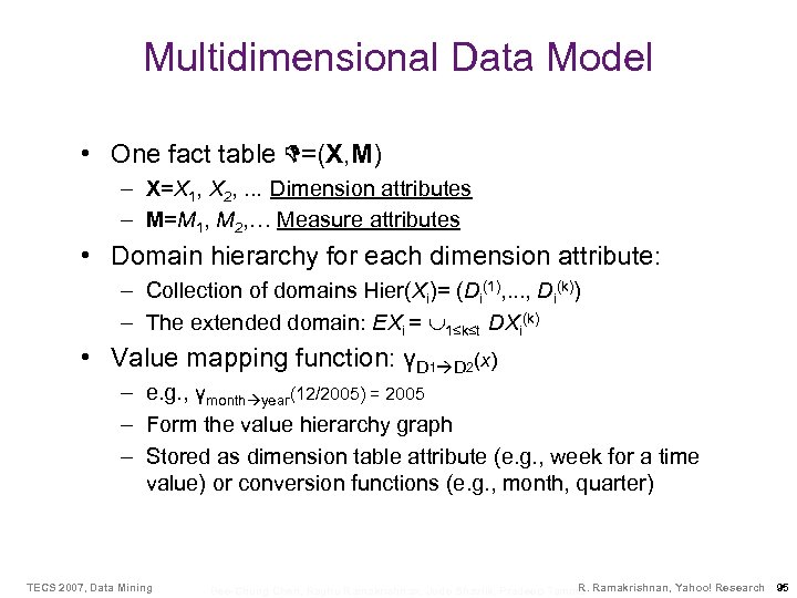
Multidimensional Data Model • One fact table D=(X, M) – X=X 1, X 2, . . . Dimension attributes – M=M 1, M 2, … Measure attributes • Domain hierarchy for each dimension attribute: – Collection of domains Hier(Xi)= (Di(1), . . . , Di(k)) – The extended domain: EXi = 1≤k≤t DXi(k) • Value mapping function: γD 1 D 2(x) – e. g. , γmonth year(12/2005) = 2005 – Form the value hierarchy graph – Stored as dimension table attribute (e. g. , week for a time value) or conversion functions (e. g. , month, quarter) TECS 2007, Data Mining R. Bee-Chung Chen, Raghu Ramakrishnan, Jude Shavlik, Pradeep Tamma Ramakrishnan, Yahoo! Research 95
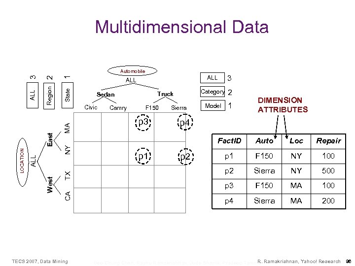
Multidimensional Data 2 1 Region State MA ALL Truck Sedan Camry F 150 p 3 Sierra 3 Category ALL Civic 2 Model 1 DIMENSION ATTRIBUTES p 4 TX TECS 2007, Data Mining Repair p 1 F 150 NY 100 Sierra NY 500 F 150 MA 100 p 4 p 2 Loc p 2 p 1 Auto p 3 NY Fact. ID CA West ALL LOCATION East 3 ALL Automobile Sierra MA 200 R. Bee-Chung Chen, Raghu Ramakrishnan, Jude Shavlik, Pradeep Tamma Ramakrishnan, Yahoo! Research 96
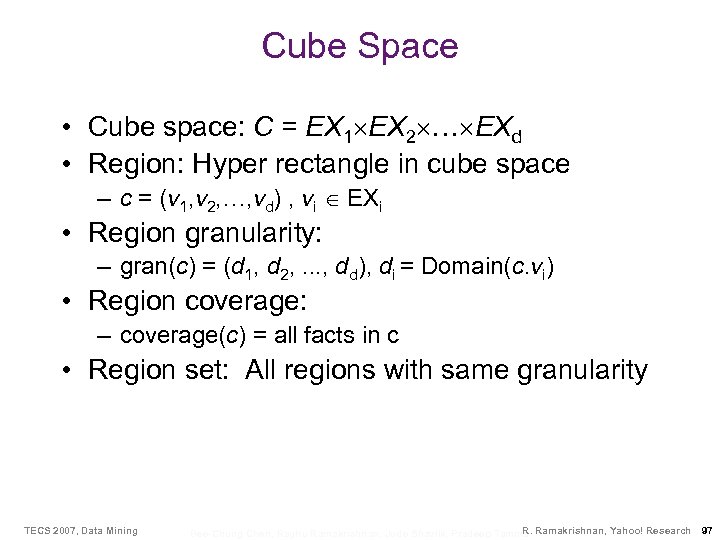
Cube Space • Cube space: C = EX 1 EX 2 … EXd • Region: Hyper rectangle in cube space – c = (v 1, v 2, …, vd) , vi EXi • Region granularity: – gran(c) = (d 1, d 2, . . . , dd), di = Domain(c. vi) • Region coverage: – coverage(c) = all facts in c • Region set: All regions with same granularity TECS 2007, Data Mining R. Bee-Chung Chen, Raghu Ramakrishnan, Jude Shavlik, Pradeep Tamma Ramakrishnan, Yahoo! Research 97
OLAP Over Imprecise Data with Doug Burdick, Prasad Deshpande, T. S. Jayram, and Shiv Vaithyanathan In VLDB 05, 06 joint work with IBM Almaden TECS 2007, Data Mining R. Bee-Chung Chen, Raghu Ramakrishnan, Jude Shavlik, Pradeep Tamma Ramakrishnan, Yahoo! Research 98
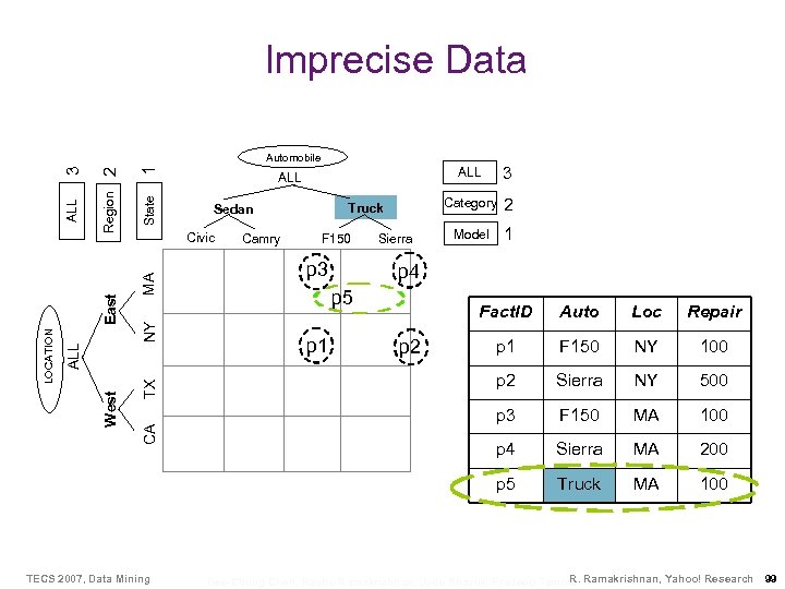
Imprecise Data 2 1 Region State ALL Truck Sedan Camry F 150 p 3 Sierra 3 Category ALL Civic MA East 3 ALL Automobile 2 Model 1 p 4 p 5 NY TX CA West ALL LOCATION Repair p 1 F 150 NY 100 Sierra NY 500 F 150 MA 100 p 4 Sierra MA 200 p 5 TECS 2007, Data Mining Loc p 3 p 2 Auto p 2 p 1 Fact. ID Truck MA 100 R. Bee-Chung Chen, Raghu Ramakrishnan, Jude Shavlik, Pradeep Tamma Ramakrishnan, Yahoo! Research 99
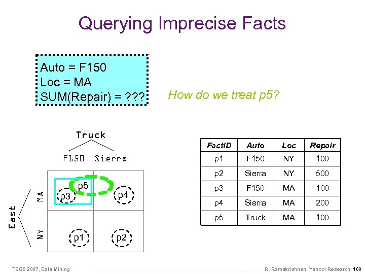
Querying Imprecise Facts Auto = F 150 Loc = MA SUM(Repair) = ? ? ? How do we treat p 5? Truck Fact. ID MA NY East p 3 TECS 2007, Data Mining p 1 p 4 Repair p 1 F 150 NY 100 Sierra NY 500 p 3 F 150 MA 100 p 4 Sierra MA 200 p 5 Sierra Loc p 2 F 150 Auto Truck MA 100 p 2 R. Bee-Chung Chen, Raghu Ramakrishnan, Jude Shavlik, Pradeep Tamma Ramakrishnan, Yahoo! Research 100
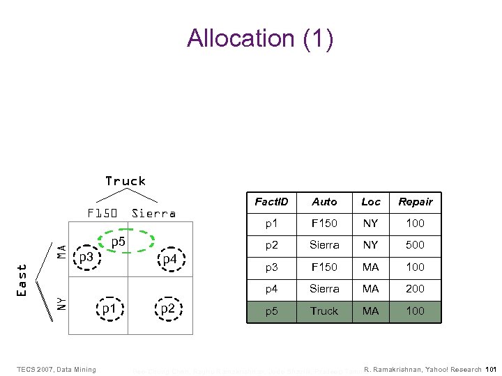
Allocation (1) Truck MA p 3 NY East p 5 TECS 2007, Data Mining p 4 p 1 p 2 Loc Repair p 1 F 150 NY 100 p 2 Sierra Auto Sierra NY 500 p 3 F 150 MA 100 p 4 F 150 Fact. ID Sierra MA 200 p 5 Truck MA 100 R. Bee-Chung Chen, Raghu Ramakrishnan, Jude Shavlik, Pradeep Tamma Ramakrishnan, Yahoo! Research 101
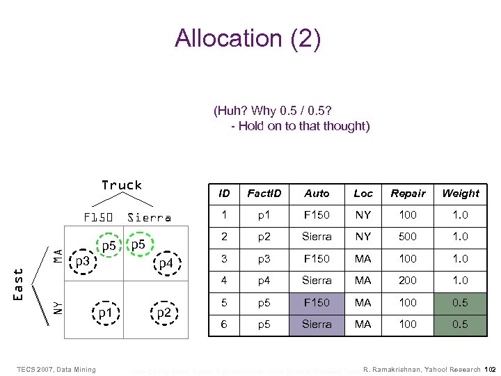
Allocation (2) (Huh? Why 0. 5 / 0. 5? - Hold on to that thought) Truck MA p 3 NY East p 5 TECS 2007, Data Mining p 5 p 4 p 1 p 2 Auto Loc Repair Weight 1 p 1 F 150 NY 100 1. 0 2 Sierra Fact. ID p 2 Sierra NY 500 1. 0 3 p 3 F 150 MA 100 1. 0 4 F 150 ID p 4 Sierra MA 200 1. 0 5 p 5 F 150 MA 100 0. 5 6 p 5 Sierra MA 100 0. 5 R. Bee-Chung Chen, Raghu Ramakrishnan, Jude Shavlik, Pradeep Tamma Ramakrishnan, Yahoo! Research 102
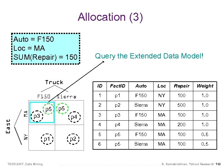
Allocation (3) Auto = F 150 Loc = MA SUM(Repair) = 150 Truck p 3 NY MA p 5 TECS 2007, Data Mining ID p 5 p 4 p 1 p 2 Auto Loc Repair Weight 1 p 1 F 150 NY 100 1. 0 2 Sierra Fact. ID p 2 Sierra NY 500 1. 0 3 p 3 F 150 MA 100 1. 0 4 F 150 East Query the Extended Data Model! p 4 Sierra MA 200 1. 0 5 p 5 F 150 MA 100 0. 5 6 p 5 Sierra MA 100 0. 5 R. Bee-Chung Chen, Raghu Ramakrishnan, Jude Shavlik, Pradeep Tamma Ramakrishnan, Yahoo! Research 103
Allocation Policies • The procedure for assigning allocation weights is referred to as an allocation policy: – Each allocation policy uses different information to assign allocation weights – Reflects assumption about the correlation structure in the data • Leads to EM-style iterative algorithms for allocating imprecise facts, maximizing likelihood of observed data TECS 2007, Data Mining R. Bee-Chung Chen, Raghu Ramakrishnan, Jude Shavlik, Pradeep Tamma Ramakrishnan, Yahoo! Research 104
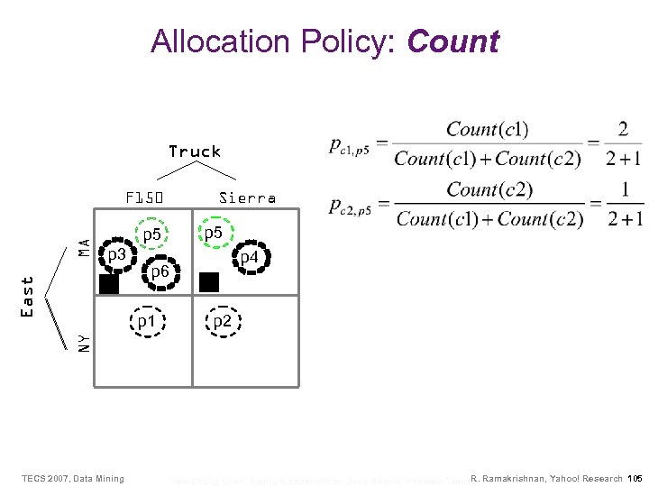
Allocation Policy: Count Truck East MA F 150 p 5 p 3 c 1 p 6 p 5 p 4 c 2 p 2 NY p 1 Sierra TECS 2007, Data Mining R. Bee-Chung Chen, Raghu Ramakrishnan, Jude Shavlik, Pradeep Tamma Ramakrishnan, Yahoo! Research 105
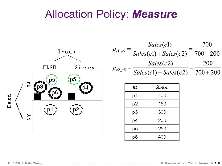
Allocation Policy: Measure Truck MA F 150 p 5 p 3 Sierra p 5 p 4 East NY TECS 2007, Data Mining 100 p 2 150 p 3 300 p 4 p 2 p 1 200 250 p 6 p 1 c 2 Sales p 5 c 1 p 6 ID 400 R. Bee-Chung Chen, Raghu Ramakrishnan, Jude Shavlik, Pradeep Tamma Ramakrishnan, Yahoo! Research 106
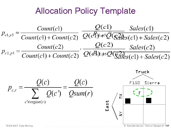
Allocation Policy Template Truck F 150 MA r c 1 c 2 NY East TECS 2007, Data Mining Sierra R. Bee-Chung Chen, Raghu Ramakrishnan, Jude Shavlik, Pradeep Tamma Ramakrishnan, Yahoo! Research 107
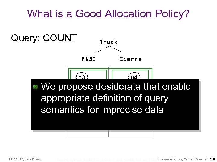
What is a Good Allocation Policy? Query: COUNT Truck F 150 p 4 We propose desiderata that enable p 5 appropriate definition of query semantics for imprecise data NY East MA p 3 Sierra TECS 2007, Data Mining p 1 p 2 R. Bee-Chung Chen, Raghu Ramakrishnan, Jude Shavlik, Pradeep Tamma Ramakrishnan, Yahoo! Research 108
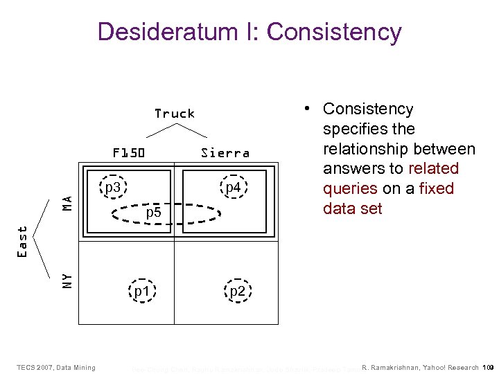
Desideratum I: Consistency Truck F 150 Sierra p 4 p 5 NY East MA p 3 • Consistency specifies the relationship between answers to related queries on a fixed data set TECS 2007, Data Mining p 1 p 2 R. Bee-Chung Chen, Raghu Ramakrishnan, Jude Shavlik, Pradeep Tamma Ramakrishnan, Yahoo! Research 109
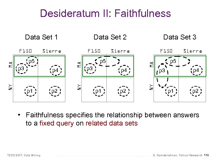
Desideratum II: Faithfulness p 3 p 4 p 1 p 2 Sierra p 5 p 3 p 4 p 1 Data Set 3 p 2 F 150 MA p 5 F 150 MA Sierra NY NY MA F 150 Data Set 2 NY Data Set 1 Sierra p 5 p 4 p 3 p 1 p 2 • Faithfulness specifies the relationship between answers to a fixed query on related data sets TECS 2007, Data Mining R. Bee-Chung Chen, Raghu Ramakrishnan, Jude Shavlik, Pradeep Tamma Ramakrishnan, Yahoo! Research 110
Results on Query Semantics • Evaluating queries over extended data model yields expected value of the aggregation operator over all possible worlds • Efficient query evaluation algorithms available for SUM, COUNT; more expensive dynamic programming algorithm for AVERAGE – Consistency and faithfulness for SUM, COUNT are satisfied under appropriate conditions – (Bound-)Consistency does not hold for AVERAGE, but holds for E(SUM)/E(COUNT) • Weak form of faithfulness holds – Opinion pooling with Lin. OP: Similar to AVERAGE TECS 2007, Data Mining R. Bee-Chung Chen, Raghu Ramakrishnan, Jude Shavlik, Pradeep Tamma Ramakrishnan, Yahoo! Research 111
![F 150 Sierra Imprecise facts lead to many possible worlds [Kripke 63, …] p F 150 Sierra Imprecise facts lead to many possible worlds [Kripke 63, …] p](https://present5.com/presentation/4303a300952882371519e116d7e110e8/image-99.jpg)
F 150 Sierra Imprecise facts lead to many possible worlds [Kripke 63, …] p 1 p 2 F 150 p 1 MA F 150 p 5 TECS 2007, Data Mining p 3 p 1 NY w 2 p 3 w 4 w 3 Sierra p 4 p 2 F 150 MA p 5 w 1 p 4 NY p 3 MA Sierra NY NY MA F 150 p 4 p 3 NY MA p 5 p 1 Sierra p 5 p 4 p 2 Sierra p 5 p 4 p 3 p 1 p 2 R. Bee-Chung Chen, Raghu Ramakrishnan, Jude Shavlik, Pradeep Tamma Ramakrishnan, Yahoo! Research 113
Query Semantics • Given all possible worlds together with their probabilities, queries are easily answered using expected values – But number of possible worlds is exponential! • Allocation gives facts weighted assignments to possible completions, leading to an extended version of the data – Size increase is linear in number of (completions of) imprecise facts – Queries operate over this extended version TECS 2007, Data Mining R. Bee-Chung Chen, Raghu Ramakrishnan, Jude Shavlik, Pradeep Tamma Ramakrishnan, Yahoo! Research 114
Exploratory Mining: Prediction Cubes with Beechun Chen, Lei Chen, and Yi Lin In VLDB 05; EDAM Project TECS 2007, Data Mining R. Bee-Chung Chen, Raghu Ramakrishnan, Jude Shavlik, Pradeep Tamma Ramakrishnan, Yahoo! Research 115
The Idea • Build OLAP data cubes in which cell values represent decision/prediction behavior – In effect, build a tree for each cell/region in the cube— observe that this is not the same as a collection of trees used in an ensemble method! – The idea is simple, but it leads to promising data mining tools – Ultimate objective: Exploratory analysis of the entire space of “data mining choices” • Choice of algorithms, data conditioning parameters … TECS 2007, Data Mining R. Bee-Chung Chen, Raghu Ramakrishnan, Jude Shavlik, Pradeep Tamma Ramakrishnan, Yahoo! Research 116
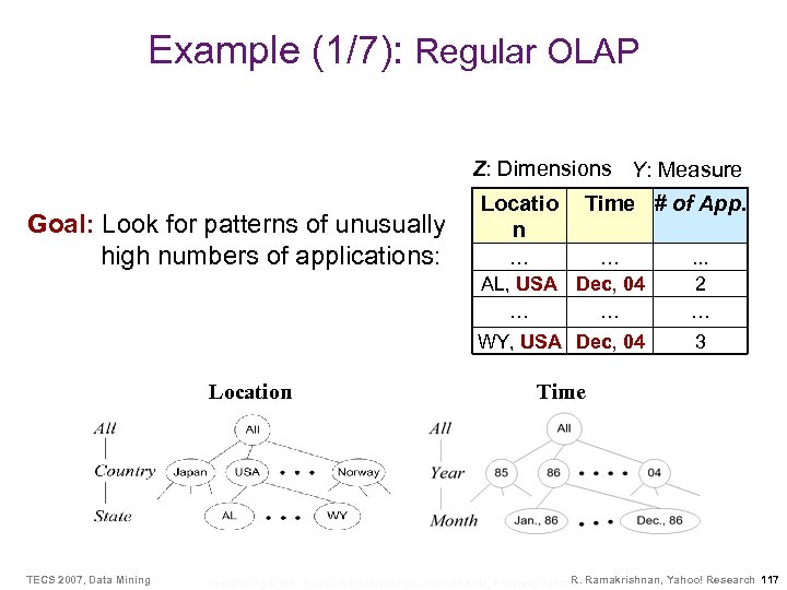
Example (1/7): Regular OLAP Z: Dimensions Y: Measure Goal: Look for patterns of unusually high numbers of applications: Locatio n Time # of App. TECS 2007, Data Mining . . . 2 … WY, USA Dec, 04 Location … … AL, USA Dec, 04 … … 3 Time R. Bee-Chung Chen, Raghu Ramakrishnan, Jude Shavlik, Pradeep Tamma Ramakrishnan, Yahoo! Research 117
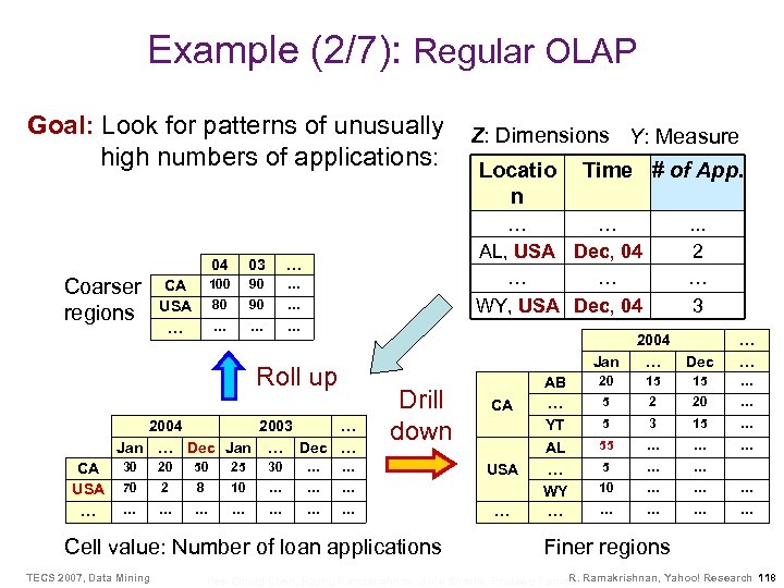
Example (2/7): Regular OLAP Goal: Look for patterns of unusually high numbers of applications: 04 Coarser regions 90 … 80 90 … … … . . . 2 … 3 Jan 2004 2003 … Jan … Dec … 30 20 50 25 30 … 70 2 8 10 … … … … CA … … Drill down … Cell value: Number of loan applications TECS 2007, Data Mining Time # of App. … Roll up CA USA … Locatio n … … AL, USA Dec, 04 … … WY, USA Dec, 04 … 100 CA USA … 03 Z: Dimensions Y: Measure USA … AB … YT AL … WY … 2004 … Dec … … 20 15 15 … 5 2 20 … 5 3 15 … 55 … … … 5 … … 10 … … … … Finer regions R. Bee-Chung Chen, Raghu Ramakrishnan, Jude Shavlik, Pradeep Tamma Ramakrishnan, Yahoo! Research 118
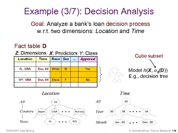
Example (3/7): Decision Analysis Goal: Analyze a bank’s loan decision process w. r. t. two dimensions: Location and Time Fact table D Z: Dimensions X: Predictors Y: Class Location Time Race Sex … AL, USA Dec, 04 White M … Yes … … … WY, USA Dec, 04 Black F … No Cube subset Approval Location TECS 2007, Data Mining Model h(X, Z(D)) E. g. , decision tree Time R. Bee-Chung Chen, Raghu Ramakrishnan, Jude Shavlik, Pradeep Tamma Ramakrishnan, Yahoo! Research 119
Example (3/7): Decision Analysis • Are there branches (and time windows) where approvals were closely tied to sensitive attributes (e. g. , race)? – • Suppose you partitioned the training data by location and time, chose the partition for a given branch and time window, and built a classifier. You could then ask, “Are the predictions of this classifier closely correlated with race? ” Are there branches and times with decision making reminiscent of 1950 s Alabama? – TECS 2007, Data Mining Requires comparison of classifiers trained using different subsets of data. R. Bee-Chung Chen, Raghu Ramakrishnan, Jude Shavlik, Pradeep Tamma Ramakrishnan, Yahoo! Research 120
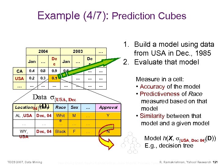
Example (4/7): Prediction Cubes 2004 2003 1. Build a model using data from USA in Dec. , 1985 2. Evaluate that model … Jan … De c … CA 0. 4 0. 8 0. 9 0. 6 0. 8 … … USA 0. 2 0. 3 0. 5 … … … Data [USA, Dec (D) Location 04]Time Race Sex … Approval AL , USA Dec, 04 … … WY, USA Whit e … M … Y … … … Dec, 04 Black F … Measure in a cell: • Accuracy of the model • Predictiveness of Race measured based on that model • Similarity between that model and a given model N TECS 2007, Data Mining Model h(X, [USA, Dec 04](D)) E. g. , decision tree R. Bee-Chung Chen, Raghu Ramakrishnan, Jude Shavlik, Pradeep Tamma Ramakrishnan, Yahoo! Research 121
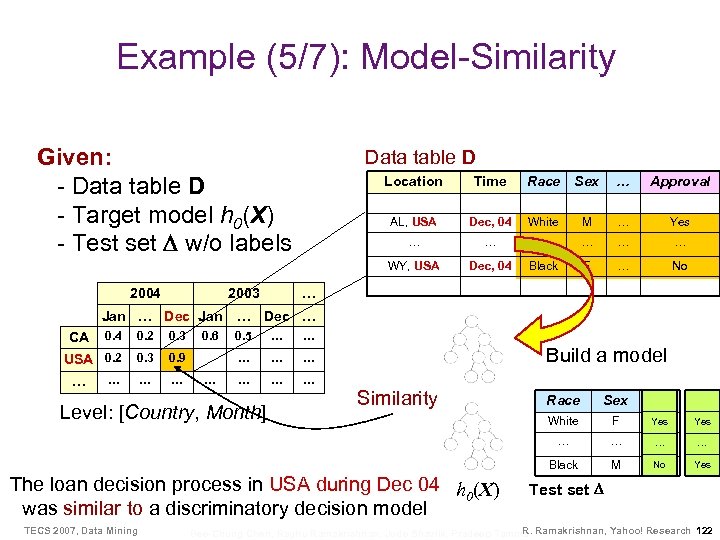
Example (5/7): Model-Similarity Given: - Data table D - Target model h 0(X) - Test set w/o labels Data table D 2003 Jan … Dec Jan 0. 4 0. 2 0. 3 USA 0. 2 0. 3 0. 9 … … … CA … 0. 6 Race Sex … Approval AL, USA Dec, 04 White M … Yes … … … Dec, 04 Black F … No … … Dec … 0. 5 … … Time WY, USA 2004 Location … … … Build a model Similarity TECS 2007, Data Mining Sex … White F Yes … … … … Black The loan decision process in USA during Dec 04 h 0(X) was similar to a discriminatory decision model Race … Level: [Country, Month] M No … Yes Test set R. Bee-Chung Chen, Raghu Ramakrishnan, Jude Shavlik, Pradeep Tamma Ramakrishnan, Yahoo! Research 122
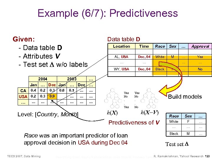
Example (6/7): Predictiveness Given: - Data table D - Attributes V - Test set w/o labels Data table D Location Time Race Sex … Approval AL, USA … Dec, 04 … White … M … … … Yes … WY, USA Dec, 04 Black F … No 2004 2003 … Jan … Dec … CA 0. 4 USA 0. 2 … … 0. 2 0. 3 0. 9 … … 0. 6 … … 0. 5 … … … Level: [Country, Month] Yes No. . Yes h(X) Yes No. . No Build models h(X V) Predictiveness of V Race was an important predictor of loan approval decision in USA during Dec 04 TECS 2007, Data Mining Race Sex … White … F … … … Black M … Test set R. Bee-Chung Chen, Raghu Ramakrishnan, Jude Shavlik, Pradeep Tamma Ramakrishnan, Yahoo! Research 123
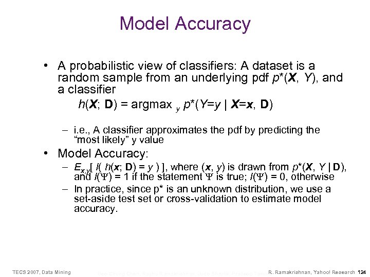
Model Accuracy • A probabilistic view of classifiers: A dataset is a random sample from an underlying pdf p*(X, Y), and a classifier h(X; D) = argmax y p*(Y=y | X=x, D) – i. e. , A classifier approximates the pdf by predicting the “most likely” y value • Model Accuracy: – Ex, y[ I( h(x; D) = y ) ], where (x, y) is drawn from p*(X, Y | D), and I( ) = 1 if the statement is true; I( ) = 0, otherwise – In practice, since p* is an unknown distribution, we use a set-aside test set or cross-validation to estimate model accuracy. TECS 2007, Data Mining R. Bee-Chung Chen, Raghu Ramakrishnan, Jude Shavlik, Pradeep Tamma Ramakrishnan, Yahoo! Research 124
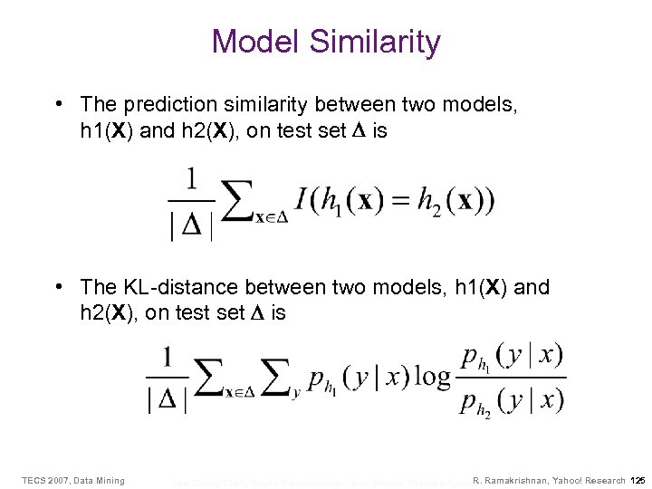
Model Similarity • The prediction similarity between two models, h 1(X) and h 2(X), on test set is • The KL-distance between two models, h 1(X) and h 2(X), on test set is TECS 2007, Data Mining R. Bee-Chung Chen, Raghu Ramakrishnan, Jude Shavlik, Pradeep Tamma Ramakrishnan, Yahoo! Research 125
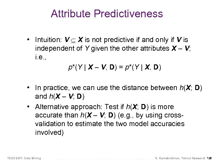
Attribute Predictiveness • Intuition: V X is not predictive if and only if V is independent of Y given the other attributes X – V; i. e. , p*(Y | X – V, D) = p*(Y | X, D) • In practice, we can use the distance between h(X; D) and h(X – V; D) • Alternative approach: Test if h(X; D) is more accurate than h(X – V; D) (e. g. , by using crossvalidation to estimate the two model accuracies involved) TECS 2007, Data Mining R. Bee-Chung Chen, Raghu Ramakrishnan, Jude Shavlik, Pradeep Tamma Ramakrishnan, Yahoo! Research 126
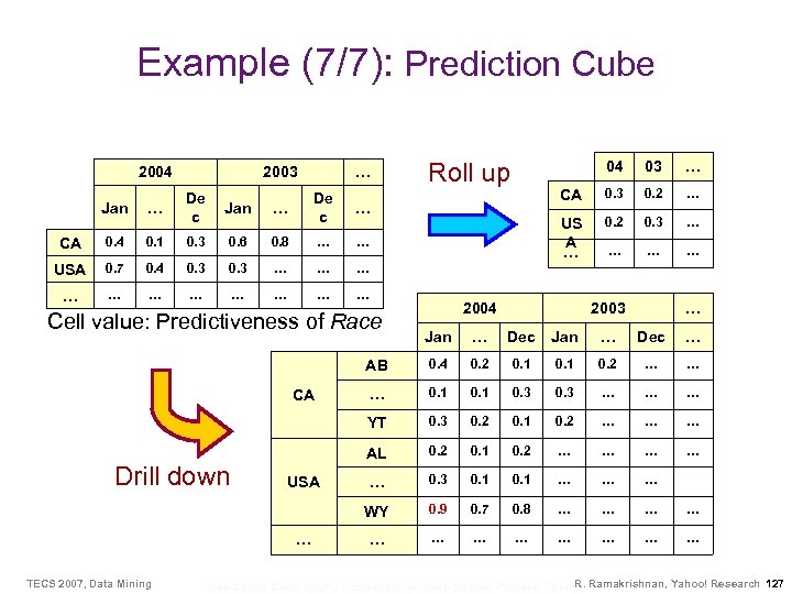
Example (7/7): Prediction Cube 2004 2003 … Jan … De c CA 0. 4 0. 1 0. 3 0. 6 0. 8 … … USA 0. 7 0. 4 0. 3 … … … … … Cell value: Predictiveness of Race … 0. 3 0. 2 … US A … … 03 CA … … 04 … Jan De c Roll up 0. 2 0. 3 … … 2004 2003 … TECS 2007, Data Mining … Dec … 0. 4 0. 2 0. 1 0. 2 … … … 0. 1 0. 3 … … … 0. 3 0. 2 0. 1 0. 2 … … … … … 0. 3 0. 1 … … … WY … Jan AL USA Dec YT Drill down … AB CA Jan 0. 9 0. 7 0. 8 … … … R. Bee-Chung Chen, Raghu Ramakrishnan, Jude Shavlik, Pradeep Tamma Ramakrishnan, Yahoo! Research 127
Efficient Computation • Reduce prediction cube computation to data cube computation – Represent a data-mining model as a distributive or algebraic (bottom-up computable) aggregate function, so that data-cube techniques can be directly applied TECS 2007, Data Mining R. Bee-Chung Chen, Raghu Ramakrishnan, Jude Shavlik, Pradeep Tamma Ramakrishnan, Yahoo! Research 128
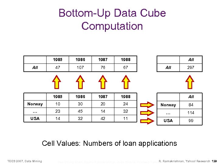
Bottom-Up Data Cube Computation 1985 1986 1987 1988 47 107 76 67 1985 1986 1987 1988 Norway 10 30 20 24 Norway 84 … 23 45 14 32 … 114 USA 14 32 42 11 USA 99 All All 297 All Cell Values: Numbers of loan applications TECS 2007, Data Mining R. Bee-Chung Chen, Raghu Ramakrishnan, Jude Shavlik, Pradeep Tamma Ramakrishnan, Yahoo! Research 129
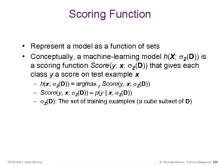
Scoring Function • Represent a model as a function of sets • Conceptually, a machine-learning model h(X; Z(D)) is a scoring function Score(y, x; Z(D)) that gives each class y a score on test example x – h(x; Z(D)) = argmax y Score(y, x; Z(D)) – Score(y, x; Z(D)) p(y | x, Z(D)) – Z(D): The set of training examples (a cube subset of D) TECS 2007, Data Mining R. Bee-Chung Chen, Raghu Ramakrishnan, Jude Shavlik, Pradeep Tamma Ramakrishnan, Yahoo! Research 130
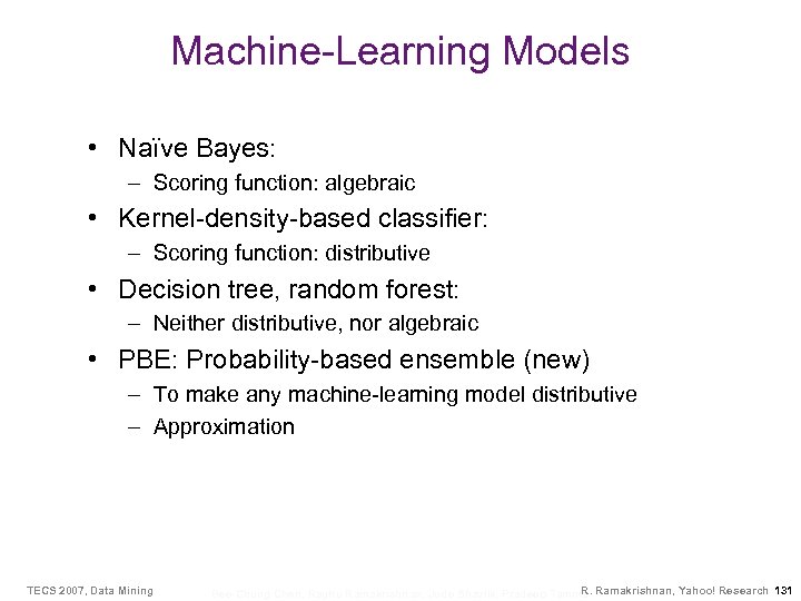
Machine-Learning Models • Naïve Bayes: – Scoring function: algebraic • Kernel-density-based classifier: – Scoring function: distributive • Decision tree, random forest: – Neither distributive, nor algebraic • PBE: Probability-based ensemble (new) – To make any machine-learning model distributive – Approximation TECS 2007, Data Mining R. Bee-Chung Chen, Raghu Ramakrishnan, Jude Shavlik, Pradeep Tamma Ramakrishnan, Yahoo! Research 131
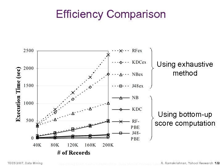
Efficiency Comparison Execution Time (sec) Using exhaustive method Using bottom-up score computation # of Records TECS 2007, Data Mining R. Bee-Chung Chen, Raghu Ramakrishnan, Jude Shavlik, Pradeep Tamma Ramakrishnan, Yahoo! Research 132
Bellwether Analysis: Global Aggregates from Local Regions with Beechun Chen, Jude Shavlik, and Pradeep Tamma In VLDB 06 TECS 2007, Data Mining R. Bee-Chung Chen, Raghu Ramakrishnan, Jude Shavlik, Pradeep Tamma Ramakrishnan, Yahoo! Research 133
Motivating Example • A company wants to predict the first year worldwide profit of a new item (e. g. , a new movie) – By looking at features and profits of previous (similar) movies, we predict expected total profit (1 -year US sales) for new movie • Wait a year and write a query! If you can’t wait, stay awake … – The most predictive “features” may be based on sales data gathered by releasing the new movie in many “regions” (different locations over different time periods). • Example “region-based” features: 1 st week sales in Peoria, week-toweek sales growth in Wisconsin, etc. • Gathering this data has a cost (e. g. , marketing expenses, waiting time) • Problem statement: Find the most predictive region features that can be obtained within a given “cost budget” TECS 2007, Data Mining R. Bee-Chung Chen, Raghu Ramakrishnan, Jude Shavlik, Pradeep Tamma Ramakrishnan, Yahoo! Research 134
Key Ideas • Large datasets are rarely labeled with the targets that we wish to learn to predict – But for the tasks we address, we can readily use OLAP queries to generate features (e. g. , 1 st week sales in Peoria) and even targets (e. g. , profit) for mining • We use data-mining models as building blocks in the mining process, rather than thinking of them as the end result – The central problem is to find data subsets (“bellwether regions”) that lead to predictive features which can be gathered at low cost for a new case TECS 2007, Data Mining R. Bee-Chung Chen, Raghu Ramakrishnan, Jude Shavlik, Pradeep Tamma Ramakrishnan, Yahoo! Research 135
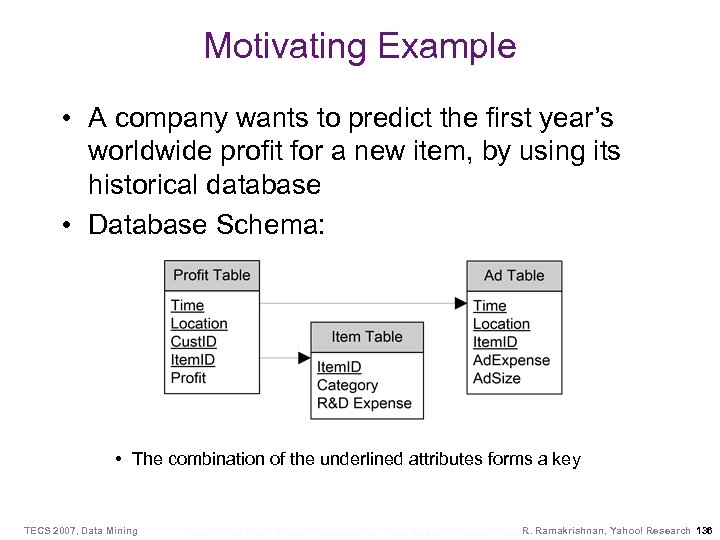
Motivating Example • A company wants to predict the first year’s worldwide profit for a new item, by using its historical database • Database Schema: • The combination of the underlined attributes forms a key TECS 2007, Data Mining R. Bee-Chung Chen, Raghu Ramakrishnan, Jude Shavlik, Pradeep Tamma Ramakrishnan, Yahoo! Research 136
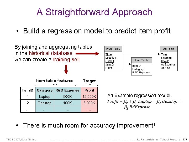
A Straightforward Approach • Build a regression model to predict item profit By joining and aggregating tables in the historical database we can create a training set: Item-table features Item. ID Category R&D Expense Target Profit 1 Laptop 500 K 12, 000 K 2 Desktop 100 K 8, 000 K … … An Example regression model: Profit = 0 + 1 Laptop + 2 Desktop + 3 Rd. Expense • There is much room for accuracy improvement! TECS 2007, Data Mining R. Bee-Chung Chen, Raghu Ramakrishnan, Jude Shavlik, Pradeep Tamma Ramakrishnan, Yahoo! Research 137
![Using Regional Features • Example region: [1 st week, HK] • Regional features: – Using Regional Features • Example region: [1 st week, HK] • Regional features: –](https://present5.com/presentation/4303a300952882371519e116d7e110e8/image-124.jpg)
Using Regional Features • Example region: [1 st week, HK] • Regional features: – Regional Profit: The 1 st week profit in HK – Regional Ad Expense: The 1 st week ad expense in HK • A possibly more accurate model: Profit[1 yr, All] = 0 + 1 Laptop + 2 Desktop + 3 Rd. Expense + 4 Profit[1 wk, KR] + 5 Ad. Expense[1 wk, KR] • Problem: Which region should we use? – The smallest region that improves the accuracy the most – We give each candidate region a cost – The most “cost-effective” region is the bellwether region TECS 2007, Data Mining R. Bee-Chung Chen, Raghu Ramakrishnan, Jude Shavlik, Pradeep Tamma Ramakrishnan, Yahoo! Research 138
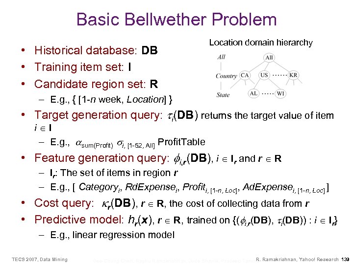
Basic Bellwether Problem • Historical database: DB • Training item set: I • Candidate region set: R Location domain hierarchy – E. g. , { [1 -n week, Location] } • Target generation query: i(DB) returns the target value of item i I – E. g. , sum(Profit) i, [1 -52, All] Profit. Table • Feature generation query: i, r(DB), i Ir and r R – Ir: The set of items in region r – E. g. , [ Categoryi, Rd. Expensei, Profiti, [1 -n, Loc], Ad. Expensei, [1 -n, Loc] ] • Cost query: r(DB), r R, the cost of collecting data from r • Predictive model: hr(x), r R, trained on {( i, r(DB), i(DB)) : i Ir} – E. g. , linear regression model TECS 2007, Data Mining R. Bee-Chung Chen, Raghu Ramakrishnan, Jude Shavlik, Pradeep Tamma Ramakrishnan, Yahoo! Research 139
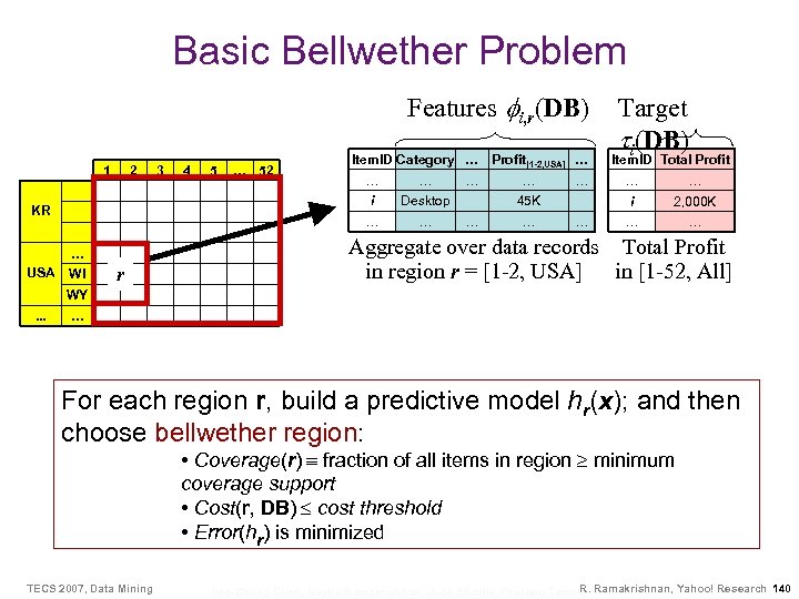
Basic Bellwether Problem Features i, r(DB) 1 2 4 5 … 52 Item. ID Category … Profit[1 -2, USA] … WI r … Desktop … … … i KR USA 3 … … … Item. ID Total Profit … … … i 45 K … Target i(DB) 2, 000 K … … Aggregate over data records Total Profit in region r = [1 -2, USA] in [1 -52, All] WY. . . … For each region r, build a predictive model hr(x); and then choose bellwether region: • Coverage(r) fraction of all items in region minimum coverage support • Cost(r, DB) cost threshold • Error(hr) is minimized TECS 2007, Data Mining R. Bee-Chung Chen, Raghu Ramakrishnan, Jude Shavlik, Pradeep Tamma Ramakrishnan, Yahoo! Research 140
![Experiment on a Mail Order Dataset Error-vs-Budget Plot [1 -8 month, MD] TECS 2007, Experiment on a Mail Order Dataset Error-vs-Budget Plot [1 -8 month, MD] TECS 2007,](https://present5.com/presentation/4303a300952882371519e116d7e110e8/image-127.jpg)
Experiment on a Mail Order Dataset Error-vs-Budget Plot [1 -8 month, MD] TECS 2007, Data Mining • Bel Err: The error of the bellwether region found using a given budget • Avg Err: The average error of all the cube regions with costs under a given budget • Smp Err: The error of a set of randomly sampled (non-cube) regions with costs under a given budget (RMSE: Root Mean Square Error) R. Bee-Chung Chen, Raghu Ramakrishnan, Jude Shavlik, Pradeep Tamma Ramakrishnan, Yahoo! Research 141
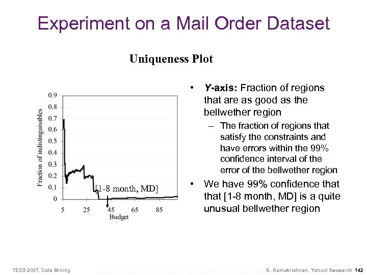
Experiment on a Mail Order Dataset Uniqueness Plot • Y-axis: Fraction of regions that are as good as the bellwether region – The fraction of regions that satisfy the constraints and have errors within the 99% confidence interval of the error of the bellwether region [1 -8 month, MD] TECS 2007, Data Mining • We have 99% confidence that [1 -8 month, MD] is a quite unusual bellwether region R. Bee-Chung Chen, Raghu Ramakrishnan, Jude Shavlik, Pradeep Tamma Ramakrishnan, Yahoo! Research 142
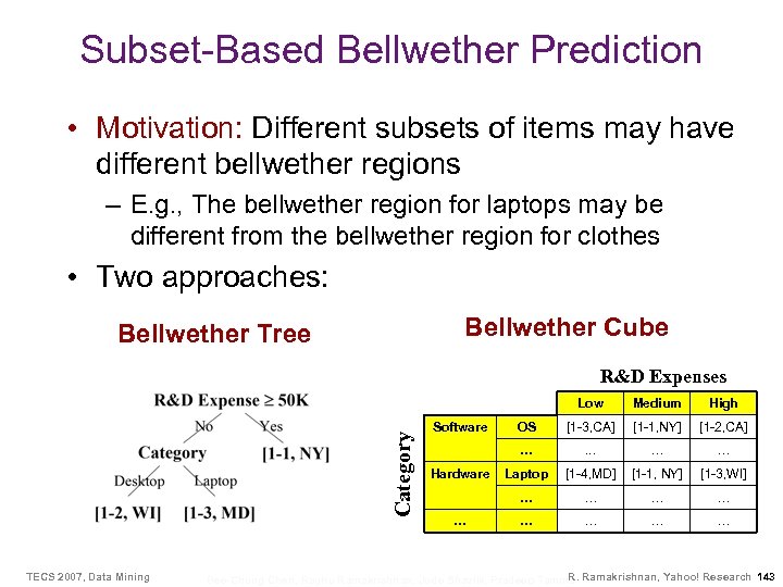
Subset-Based Bellwether Prediction • Motivation: Different subsets of items may have different bellwether regions – E. g. , The bellwether region for laptops may be different from the bellwether region for clothes • Two approaches: Bellwether Cube Bellwether Tree R&D Expenses Category Low TECS 2007, Data Mining … OS [1 -3, CA] [1 -1, NY] [1 -2, CA] . . . … … Laptop [1 -4, MD] [1 -1, NY] [1 -3, WI] … Hardware High … Software Medium … … … … R. Bee-Chung Chen, Raghu Ramakrishnan, Jude Shavlik, Pradeep Tamma Ramakrishnan, Yahoo! Research 143
Bellwether Analysis Conclusions TECS 2007 R. Ramakrishnan, Yahoo! Research
![Related Work: Building models on OLAP Results • Multi-dimensional regression [Chen, VLDB 02] – Related Work: Building models on OLAP Results • Multi-dimensional regression [Chen, VLDB 02] –](https://present5.com/presentation/4303a300952882371519e116d7e110e8/image-131.jpg)
Related Work: Building models on OLAP Results • Multi-dimensional regression [Chen, VLDB 02] – Goal: Detect changes of trends – Build linear regression models for cube cells • Step-by-step regression in stream cubes [Liu, PAKDD 03] • Loglinear-based quasi cubes [Barbara, J. IIS 01] – Use loglinear model to approximately compress dense regions of a data cube • Net. Cube [Margaritis, VLDB 01] – Build Bayes Net on the entire dataset of approximate answer count queries TECS 2007, Data Mining R. Bee-Chung Chen, Raghu Ramakrishnan, Jude Shavlik, Pradeep Tamma Ramakrishnan, Yahoo! Research 145
![Related Work (Contd. ) • Cubegrades [Imielinski, J. DMKD 02] – Extend cubes with Related Work (Contd. ) • Cubegrades [Imielinski, J. DMKD 02] – Extend cubes with](https://present5.com/presentation/4303a300952882371519e116d7e110e8/image-132.jpg)
Related Work (Contd. ) • Cubegrades [Imielinski, J. DMKD 02] – Extend cubes with ideas from association rules – How does the measure change when we rollup or drill down? • Constrained gradients [Dong, VLDB 01] – Find pairs of similar cell characteristics associated with big changes in measure • User-cognizant multidimensional analysis [Sarawagi, VLDBJ 01] – Help users find the most informative unvisited regions in a data cube using max entropy principle • Multi-Structural DBs [Fagin et al. , PODS 05, VLDB 05] TECS 2007, Data Mining R. Bee-Chung Chen, Raghu Ramakrishnan, Jude Shavlik, Pradeep Tamma Ramakrishnan, Yahoo! Research 146
Take-Home Messages • Promising exploratory data analysis paradigm: – Can use models to identify interesting subsets – Concentrate only on subsets in cube space • Those are meaningful subsets, tractable – Precompute results and provide the users with an interactive tool • A simple way to plug “something” into cube-style analysis: – Try to describe/approximate “something” by a distributive or algebraic function TECS 2007, Data Mining R. Bee-Chung Chen, Raghu Ramakrishnan, Jude Shavlik, Pradeep Tamma Ramakrishnan, Yahoo! Research 147
Big Picture • Why stop with decision behavior? Can apply to other kinds of analyses too • Why stop at browsing? Can mine prediction cubes in their own right • Exploratory analysis of mining space: – Dimension attributes can be parameters related to algorithm, data conditioning, etc. – Tractable evaluation is a challenge: • Large number of “dimensions”, real-valued dimension attributes, difficulties in compositional evaluation • Active learning for experiment design, extending compositional methods TECS 2007, Data Mining R. Bee-Chung Chen, Raghu Ramakrishnan, Jude Shavlik, Pradeep Tamma Ramakrishnan, Yahoo! Research 148
4303a300952882371519e116d7e110e8.ppt