ec1f5a11fc7c5816ef88bef0605f31b6.ppt
- Количество слайдов: 63
Behavioural Finance Lecture 08 Out of Sequence… Behavioural Finance and Economics 01
An out of sequence lecture… • Would have covered experiments in behavioural finance – But research with CSIRO this week left no time – Jumping one week forward • Impact of behavioural finance on macroeconomics • Statistics on money & implications for economic theory – New, credit-driven theory of macroeconomics • First, overview of implications of behavioural finance for how we “do” economics… – If agents not “rational” as neoclassicals define it • Able to predict future accurately! – Then economics and finance can’t be separated…
Behavioural vs Neoclassical Finance • CAPM’s Modigliani-Miller “Dividend Irrelevance Theorem” – Argued debt didn’t affect value of company – Theorem also falls with failure of CAPM – Debt matters for value of company – Debt also affects economic performance • MM theorem neatly divided economics & finance – Finance studied firms/individuals/asset values without considering macroeconomics – Economics studied macro economy without considering finance • Since CAPM false, economics & finance must be studied together… – Question is, how to study them?
Behavioural vs Neoclassical Finance • Neoclassical economics emphasises “rational agent” – Where rational means “able to predict future”! • Behavioural economics emphasises “irrational behaviour” – Also Simons emphasises “bounded rationality” • Both imply model economy using “limited cognition” agents • But there’s another alternative – Don’t use agents at all! • Many sciences involve interacting “agents” – E. g. , biology – Most biological models don’t use “agents” but “populations” • E. g. , “predator-prey” models…
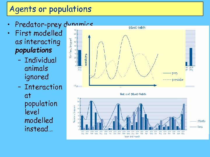
Agents or populations • Predator-prey dynamics… • First modelled as interacting populations – Individual animals ignored – Interaction at population level modelled instead…
Behavioural vs Neoclassical Finance • Emphasis on agents rather than populations may have handicapped economics – Economy a very complex system – Individual agents “know” only very limited parts of it – Structure of economy may be more important than decisions of isolated agents – Relations between agents (known & unknown) may be more important than actions of individuals themselves • Witness “demand curve can have any shape at all” dilemma when generalising from one consumer to many in a single market • So structural, “tops-down” modelling may tell us more than modelling individual agents – Even if agents modelled as “satisficers” not optimisers
Behavioural vs Neoclassical Finance • Way forward may be – build “population level” models first – Develop “agent-based” models later if desired • Where both replicate empirical data • Essential therefore to “know the data” on economics & finance – Excellent study on this by Kydland & Prescott 1990… • This lecture—consider what data implies for model of economy • Next 4 lectures: build dynamic, credit-driven model of economy
What’s the link between economics & finance? • Standard view: there is none! – Economics to Finance: • IS-LM macroeconomics (both Keynesian & Neoclassical) – Money supply exogenous—set by Central Bank – Changing money supply changes interest rate – No other link between economics & finance – Finance to Economics: • Efficient markets hypothesis (EMH): – Firm’s value set by NPV of expected cash flow from investments – How firm finances investments has no impact on its value – Therefore finance has no impact on the economy
What’s the link between economics & finance? • In this subject, we ask: – What does the data show? • Data strongly contradicts standard IS-LM and CAPM – Empirical failure of CAPM now widely acknowledged – Empirical problems with IS-LM also widely known, but • Still no accepted alternative to either – In this subject, we • Consider the data • Evaluate standard theories against it • Introduce new theories that better match the data – First, recap of conventional views of money & finance…
Money & Economics, Finance & Expectations • Dominant view: money simply a “veil over barter” – Facilitates exchange of goods, but… • No long-term impact (“money neutrality”) • Perhaps some short-term impact on prices… – Barter economy minus “double coincidence of wants” • Consumer A has commodity X & wants Y • Consumer B has commodity Y & wants X • Without money – A & B have to “find each other” to exchange • With money – A sells X for $ market price, buys Y – B sells Y for $ market price , buys X – Money commodity a “convenient numeraire”
“Veil over barter” • “Veil over barter” view dominates macro & finance theory – Economics: “quantity theory of money” (MV=PT) • Money supply exogenously controlled by government • Inflation caused by too rapid increase in money supply w. r. t rate of growth of economy • Output and price sides of economy independent – Short term effect of expansionary policy under Friedman’s “adaptive expectations” • Vertical long run Phillips Curve – No effect of government at all under “rational expectations” • Vertical short run Phillips Curve
Standard model of money creation • Government (Reserve Bank) creates “high powered money” (money base B & M 1) – Notes and coins – Government deficit • High powered money deposited in private bank accounts • “Money multiplier” ratio m between base & broad money determines amount of money (M 2, M 3, etc. ) • In quantitative control days, m set by policy – Banks required to keep set percentage m of deposits in reserve • Now m set indirectly by Basel accords (risk rating of different classes of bank investments) • But mechanics the same however m set…
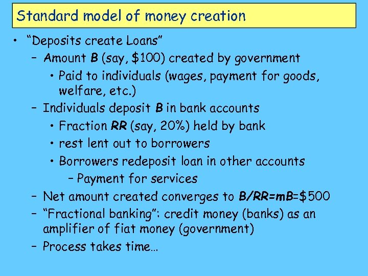
Standard model of money creation • “Deposits create Loans” – Amount B (say, $100) created by government • Paid to individuals (wages, payment for goods, welfare, etc. ) – Individuals deposit B in bank accounts • Fraction RR (say, 20%) held by bank • rest lent out to borrowers • Borrowers redeposit loan in other accounts – Payment for services – Net amount created converges to B/RR=m. B=$500 – “Fractional banking”: credit money (banks) as an amplifier of fiat money (government) – Process takes time…
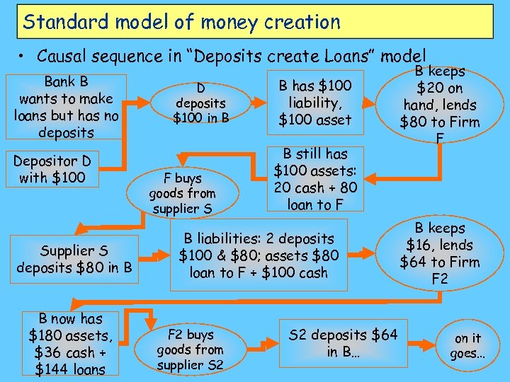
Standard model of money creation • Causal sequence in “Deposits create Loans” model Bank B wants to make loans but has no deposits Depositor D with $100 Supplier S deposits $80 in B B now has $180 assets, $36 cash + $144 loans D deposits $100 in B F buys goods from supplier S B has $100 liability, $100 asset B still has $100 assets: 20 cash + 80 loan to F B liabilities: 2 deposits $100 & $80; assets $80 loan to F + $100 cash F 2 buys goods from supplier S 2 deposits $64 in B… B keeps $20 on hand, lends $80 to Firm F B keeps $16, lends $64 to Firm F 2 on it goes…
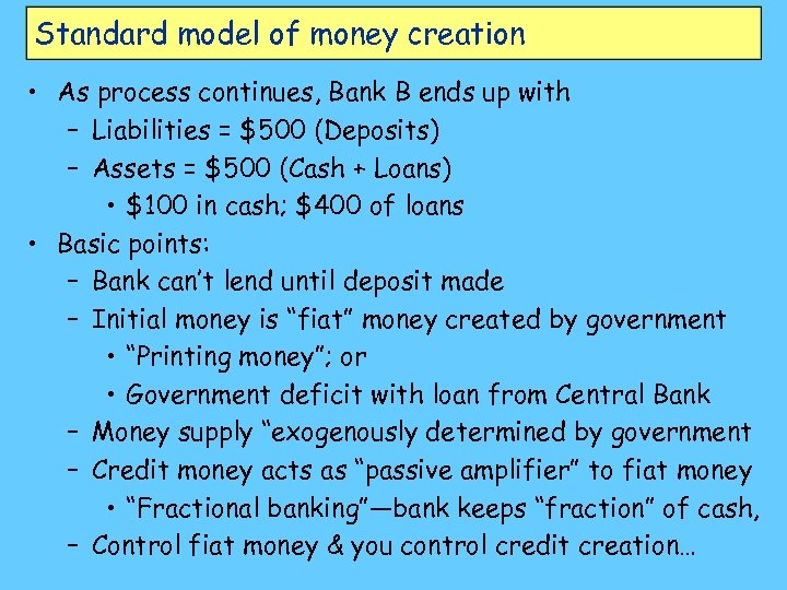
Standard model of money creation • As process continues, Bank B ends up with – Liabilities = $500 (Deposits) – Assets = $500 (Cash + Loans) • $100 in cash; $400 of loans • Basic points: – Bank can’t lend until deposit made – Initial money is “fiat” money created by government • “Printing money”; or • Government deficit with loan from Central Bank – Money supply “exogenously determined by government – Credit money acts as “passive amplifier” to fiat money • “Fractional banking”—bank keeps “fraction” of cash, – Control fiat money & you control credit creation…
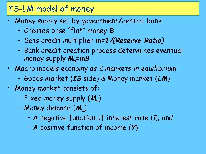
IS-LM model of money • Money supply set by government/central bank – Creates base “fiat” money B – Sets credit multiplier m=1/(Reserve Ratio) – Bank credit creation process determines eventual money supply Ms=m. B • Macro models economy as 2 markets in equilibrium: – Goods market (IS side) & Money market (LM) • Money market consists of: – Fixed money supply (Ms) – Money demand (Md) • A negative function of interest rate (i); and • A positive function of income (Y)
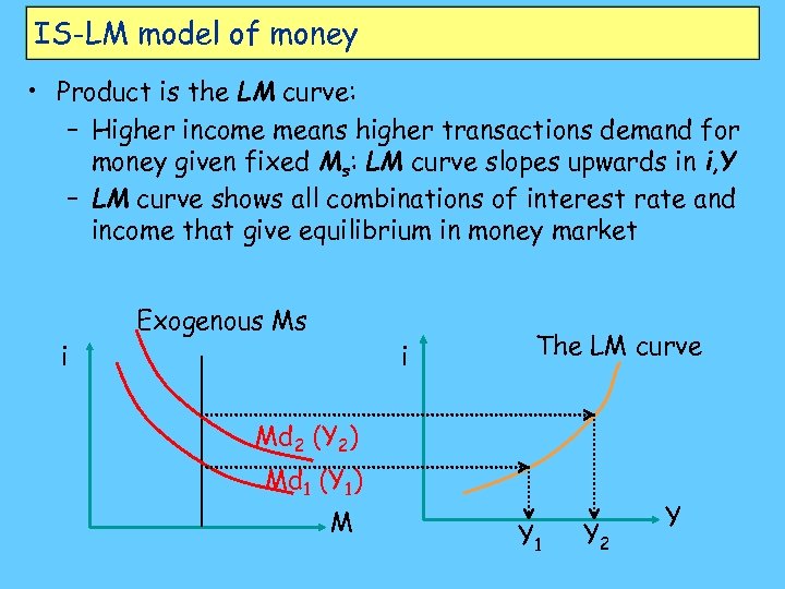
IS-LM model of money • Product is the LM curve: – Higher income means higher transactions demand for money given fixed Ms: LM curve slopes upwards in i, Y – LM curve shows all combinations of interest rate and income that give equilibrium in money market i Exogenous Ms i The LM curve Md 2 (Y 2) Md 1 (Y 1) M Y 1 Y 2 Y
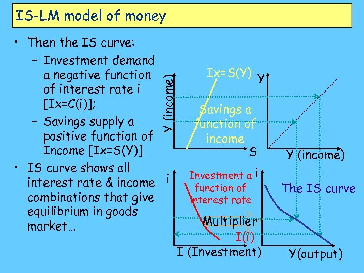
IS-LM model of money Y (income) • Then the IS curve: – Investment demand a negative function of interest rate i [Ix=C(i)]; – Savings supply a positive function of Income [Ix=S(Y)] • IS curve shows all interest rate & income i combinations that give equilibrium in goods market… Ix=S(Y) Y Savings a function of income S Investment a i function of interest rate Multiplier I(i) I (Investment) Y (income) The IS curve Y(output)
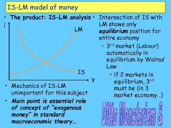
IS-LM model of money • The product: IS-LM analysis • Intersection of IS with LM shows only i LM equilibrium position for entire economy – 3 rd market (Labour) automatically in equilibrium by Walras’ Law IS • if 2 markets in Y equilibrium, 3 rd • Mechanics of IS-LM must be (in 3 unimportant for this subject market economy…) • Main point is essential role of concept of “exogenous money” in standard macroeconomic theory…
Efficient Markets Hypothesis model of finance • Finance markets efficiently price risk & return of assets… – “Assets which are unaffected by changes in economic activity will return the pure interest rate; those which move with economic activity will promise appropriately higher expected rates of return. ” (Sharpe 1964) • Financing of firms doesn’t affect value… • “We conclude therefore that levered companies cannot command a premium over unlevered companies because investors have the opportunity of putting the equivalent leverage into their portfolio directly by borrowing on personal account. ” (Modigliani-Miller) • Stock market returns follow a random walk… – Which we already know is empirically false (see Fractal Markets lecture)
Opposing view: money “fundamentally different” • Money economy “fundamentally different” to barter system • Money originates in credit extended by banks – Money necessarily has debt associated with it – Quantity of money & debt impacts on real economy • Not just “price level” effects but – Short run & Long run impacts on output, employment, etc. • Starts from different vision of purpose of trade – “Veil over barter” vision • Object of trade is consumption – “Fundamentally different” vision • Object of trade is accumulation of wealth
Opposing view: money “fundamentally different” • Best statement of “veil over barter vision” by Say: – “Every producer asks for money in exchange for his products, only for the purpose of employing that money again immediately in the purchase of another product; for we do not consume money, and it is not sought after in ordinary cases to conceal it: …. It is thus that the producers, though they have all of them the air of demanding money for their goods, do in reality demand merchandise for their merchandise. ” (Jean Baptiste Say, Catechism of Political Economy). • Best statement of “accumulation vision” by Marx – Veil over barter argues traders exchange goods they have & don’t want for those they don’t have & do want • Marx agrees… “So far as regards use-values, it is clear that both parties may gain some advantage. ”
“Fundamentally different”: Marx • With reference , therefore, to use-value, there is good ground for saying that 'exchange is a transaction by which both sides gain. ‘” (Capital I Ch. 5) • But this isn’t the “main game”: – “It must never be forgotten, that in capitalist production what matters is not the immediate usevalue but the exchange-value, and, in particular, the expansion of surplus-value – This is the driving motive of capitalist production, and it is a pretty conception that—in order to reason away the contradictions of capitalist production—abstracts from its very basis and depicts it as a production aiming at the direct satisfaction of the consumption of the producers. ” (Theories of Surplus Value II, s 17. 6) • Money the ultimate form of accumulated wealth
“Fundamentally different”: Keynes • Keynes also derided conventional “veil over barter” view – Veil over barter asserts money gives holder no utility in itself • Say: “for we do not consume money…” – But Keynes says “utility” of money is security it gives to holders in uncertain world • Sending up conventional view, Keynes says… – “Money, it is well known, serves two principal purposes. By acting as a money of account it facilitates exchanges … In the second place, it is a store of wealth…” • Keynes continues…
“Fundamentally different”: Keynes • So we are told, without a smile on the face. But in the world of the classical economy, what an insane use to which to put it! For … money … is barren; whereas practically every other form of storing wealth yields some interest or profit. Why should anyone outside a lunatic asylum wish to use money as a store of wealth? Because, partly on reasonable and partly on instinctive grounds, our desire to hold Money as a store of wealth is a barometer of the degree of our distrust of our own calculations and conventions concerning the future…” (Keynes 1937) future… • So money “essentially different” to commodities – In a crisis, hoard of any given commodity can be worthless – Hoard of money always valuable… – Also different view of how money created…
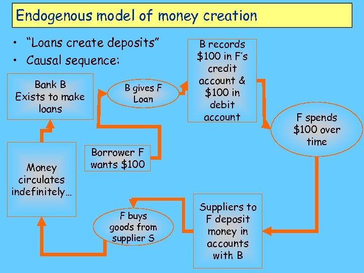
Endogenous model of money creation • “Loans create deposits” • Causal sequence: Bank B Exists to make loans Money circulates indefinitely… B gives F Loan B records $100 in F’s credit account & $100 in debit account Borrower F wants $100 F buys goods from supplier S Suppliers to F deposit money in accounts with B F spends $100 over time
Rival models of money creation • In this model, credit money independent of “fiat” money – Credit money created by banking system – Fiat money created by government – Both stored in private bank accounts • Government may try to force some correspondence between them – Set target m for M: B ratio – But prime responsibility of Central Bank is ensuring financial system remains solvent – Need for systemic liquidity may mean that • “credit money M drives fiat money B”…
Rival models of money creation • So two rival models – Exogenous • Government controls money supply – Credit system simply amplifies what government does – Inflation caused by excess money supply growth – Endogenous • Credit money created by banking system – “Credit dog wags the government fiat money tail” • Central Bank forced to accommodate credit demands of corporate/financial system
And the data says? • Can the data help decide which approach is correct? • If the money supply is exogenous, then – It should not be influenced by the real economy – Changes in the stock of money should either • Have no effect on the real economy (“exogenous and irrelevant”); or • Have no effect on the real economy, but alter the price system (“exogenous and inflationary”); or – Changes in narrow, government controlled component of money supply (M 1) should precede & cause changes in broader components (M 2 & M 3) – What does the data show? • Economic data: Kydland Prescott (1990)
Kydland Prescott’s analysis • Looked at timing of economic variables to conclude what can cause what – If Y follows X in time, then Y cannot cause X – For money to be exogenous, it must be either • Uncorrelated to real and price variables; or • Correlated to real or price variables, and leading them rather than lagging them. • They concluded: "There is no evidence that either the monetary base or M 1 leads the cycle, although some economists still believe this monetary myth. Both the monetary base and M 1 series are generally procyclical, and, if anything, the monetary base lags the cycle slightly. " (14) slightly – Thus even M 1 is endogenous (determined by the economic system, not the government): how else could changes in M 1 lag changes in output?
Kydland Prescott’s analysis • Authors’ aim was data exploration – "reporting the facts—without assuming the data is generated by some probability distribution—is an important scientific activity. We see no reason for economics to be an exception" (3) • Choice of variables and expectations of relationships between variables driven by neoclassical theory (which normally assumes an exogenous money supply), but… – "The purpose of this article is to present business cycle facts in light of established neoclassical growth theory… Do the corresponding statistics for the model economy display these patterns [found in the data]? We find these features interesting because the patterns they seem to display are inconsistent with theory. " (4)
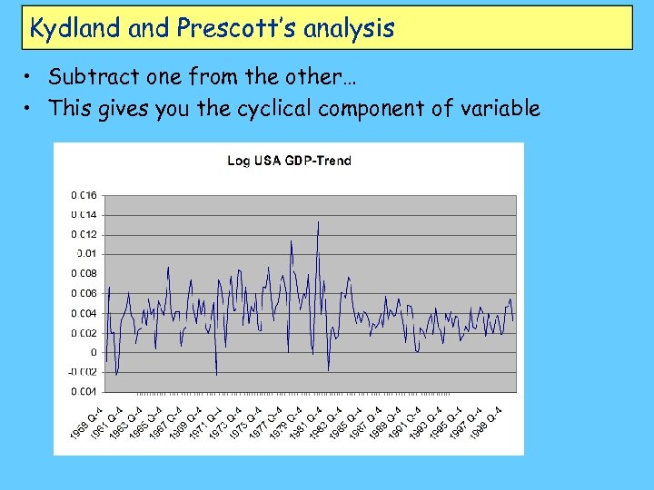
Kydland Prescott’s analysis • Use very simple definition of cycles: – "We follow Lucas in defining business cycles as the deviations of aggregate real output from trend. We complete his definition by providing an explicit procedure for calculating a time series trend that successfully mimics the smooth curves most business cycle researchers would draw through plots of the data. " (4) • Derided definitions which give causal dynamic to cycle: – Mitchell notes that "'most current theories explain crises by what happens during prosperity and revivals by what happens in depression'" (5)
Kydland Prescott’s analysis • They comment – "Theories with deterministic cyclical laws of motion may a priori have had considerable potential for accounting for business cycles; but in fact they have failed to do so. – They have failed because cyclical laws of motion do not arise as equilibrium behaviour for economics with empirically reasonable preferences and technologies— that is, for economies with reasonable statements about people's ability and willingness to substitute. " (5) • So causal cycle theories rejected on basis of economic theory of optimising agents… – However, results consonant with modern theories of deterministic cycles (as discussed in later lectures)
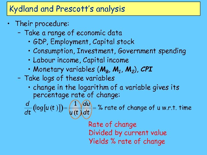
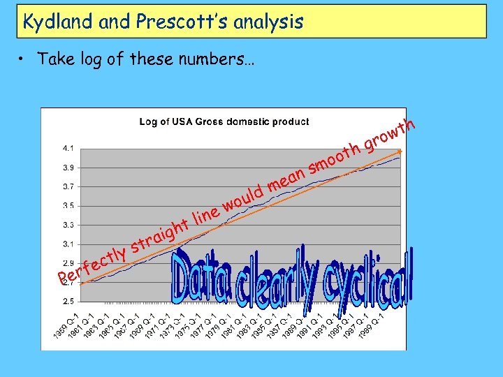
Kydland Prescott’s analysis • Their procedure: – Take a range of economic data • GDP, Employment, Capital stock • Consumption, Investment, Government spending • Labour income, Capital income • Monetary variables (MB, M 1, M 2), CPI – Take logs of these variables • change in the logarithm of a variable gives its percentage rate of change: Rate of change Divided by current value Yields % rate of change
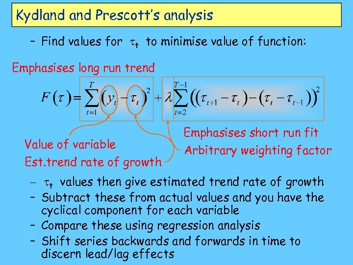
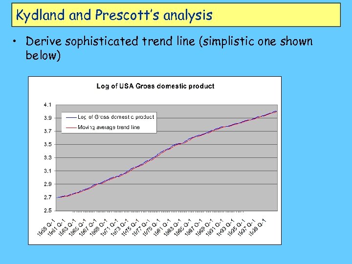
Kydland Prescott’s analysis – Find values for tt to minimise value of function: Emphasises long run trend Value of variable Est. trend rate of growth Emphasises short run fit Arbitrary weighting factor – tt values then give estimated trend rate of growth – Subtract these from actual values and you have the cyclical component for each variable – Compare these using regression analysis – Shift series backwards and forwards in time to discern lead/lag effects
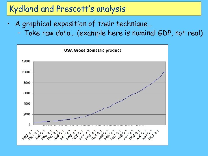
Kydland Prescott’s analysis • A graphical exposition of their technique… – Take raw data… (example here is nominal GDP, not real)
Kydland Prescott’s analysis • Take log of these numbers… oth o m ns ea line ght i erf P a str y ctl e ld m wou g wth ro
Kydland Prescott’s analysis • Derive sophisticated trend line (simplistic one shown below)
Kydland Prescott’s analysis • Subtract one from the other… • This gives you the cyclical component of variable
Kydland Prescott’s analysis • Repeat process with another variable, say investment…
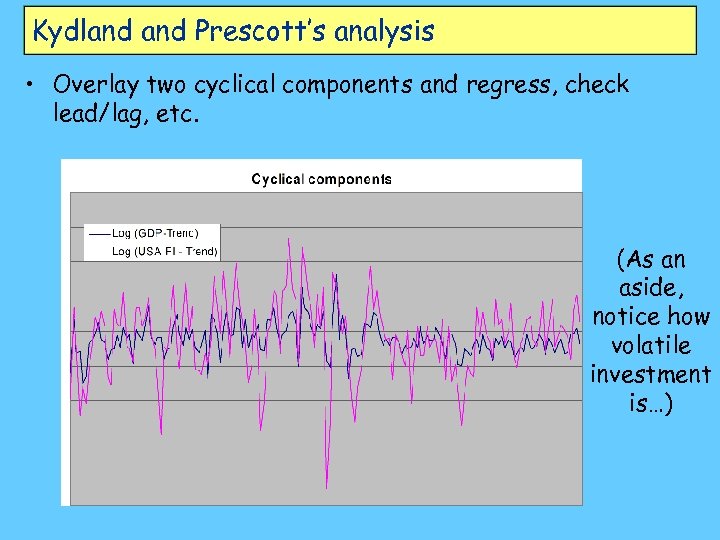
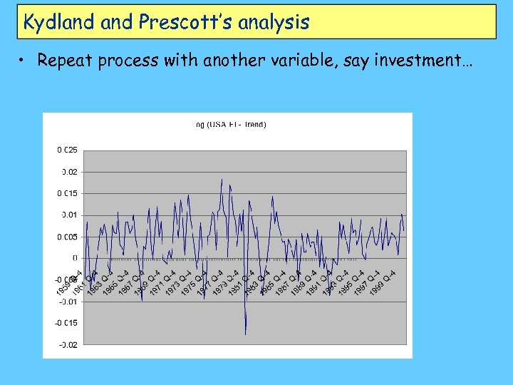
Kydland Prescott’s analysis • Overlay two cyclical components and regress, check lead/lag, etc. (As an aside, notice how volatile investment is…)
Kydland Prescott’s conclusions re money • "This finding that the real wage behaves in a reasonably strong procyclical manner is counter to a widely held belief in the literature. " (13 -14) – (Not relevant just yet, but issue comes in to play in later lectures on modelling endogenous money) • “The chart [4] shows that the bulk of the volatility in aggregate output is due to investment expenditures. ” (14) – A Keynesian perspective, despite neoclassical leanings of authors • "There is no evidence that either the monetary base or M 1 leads the cycle, although some economists still believe this monetary myth. Both the monetary base and M 1 series are generally procyclical, and, if anything, the monetary base lags the cycle slightly. " (14) – So M 1 lags the cycle…
Kydland Prescott’s conclusions re money • "The difference in the behaviour of M 1 and M 2 suggests that the difference of these aggregates (M 2 minus M 1) should be considered. This component mainly consists of interest-bearing time deposits, including certificates of deposit under $100, 000. It is approximately one-half of annual GDP, whereas M 1 is about one-sixth. The difference of M 2 -M 1 leads the cycle by even more than M 2 with the lead being about three quarters. ” • From Table 4 it is also apparent that money velocities are procyclical and quite volatile. " (17) – M 2 leads the cycle, while M 1 lags it • Then how can M 1 “cause” M 2, which is the presumption of exogenous money theory? – Again, despite neoclassical leanings of authors, results and conclusions support non-neoclassical perspectives
Kydland Prescott’s conclusions re money • "The fact that the transaction component of real cash balances (M 1) moves contemporaneously with the cycle while the much larger nontransaction component (M 2) leads the cycle suggests that credit arrangements could play a significant role in future business cycle theory. Introducing money and credit into growth theory in a way that accounts for the cyclical behaviour of monetary as well as real aggregates is an important open problem in economics. " (17) – So we need a theory in which credit plays an essential role • “From Table 4 it is also apparent that money velocities are procyclical and quite volatile. ” (17) – So much for a stable V in the MV=PT truism
Kydland Prescott’s conclusions re money • “This myth [that the price level is always procyclical] originated in the fact that, during the period between the world wars, the price level was procyclical… The fact is, however, that … the U. S. price level has been countercyclical in the post-Korean War period. ” (17) – Yet another puzzle to explain… • So the data – Does not support the proposition that M 1 controls the broad money supply • In fact the reverse seems to be the case – Does not support the proposition that V is stable • (An essential assumption of the quantity theory of money and the “money supply increases cause inflation” argument)
Kydland Prescott’s conclusions re money – Does not support the idea that high employment and high economic activity leads to price inflation – Does suggest that income distribution dynamics form part of the trade cycle – Does suggest that credit (and hence debt) plays a major role in the trade cycle • All of which points to money – being endogenous, not exogenous – interacting with real variables, not simply determining inflation – having causations in the reverse direction to conventional economic theory – Reverse causation applies in Post Keynesian theory… • In conclusion, some simple statistics on credit today…
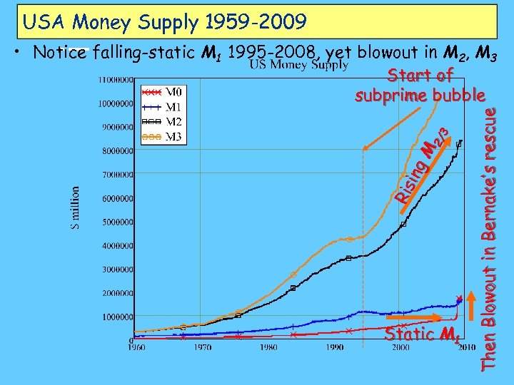
USA Money Supply 1959 -2009 Static M 1 Then Blowout in Bernake’s rescue Ris ing M 2/ 3 • Notice falling-static M 1 1995 -2008, yet blowout in M 2, M 3 Start of subprime bubble
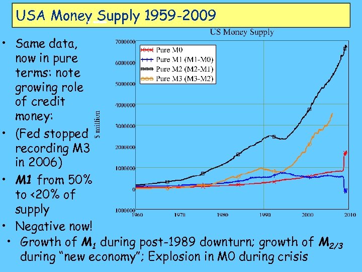
USA Money Supply 1959 -2009 • Same data, now in pure terms: note growing role of credit money: • (Fed stopped recording M 3 in 2006) • M 1 from 50% to <20% of supply • Negative now! • Growth of M 1 during post-1989 downturn; growth of M 2/3 during “new economy”; Explosion in M 0 during crisis
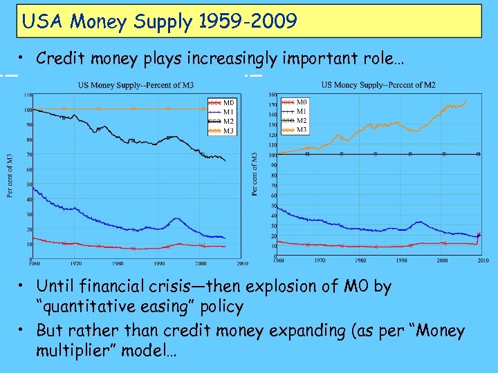
USA Money Supply 1959 -2009 • Credit money plays increasingly important role… • Until financial crisis—then explosion of M 0 by “quantitative easing” policy • But rather than credit money expanding (as per “Money multiplier” model…
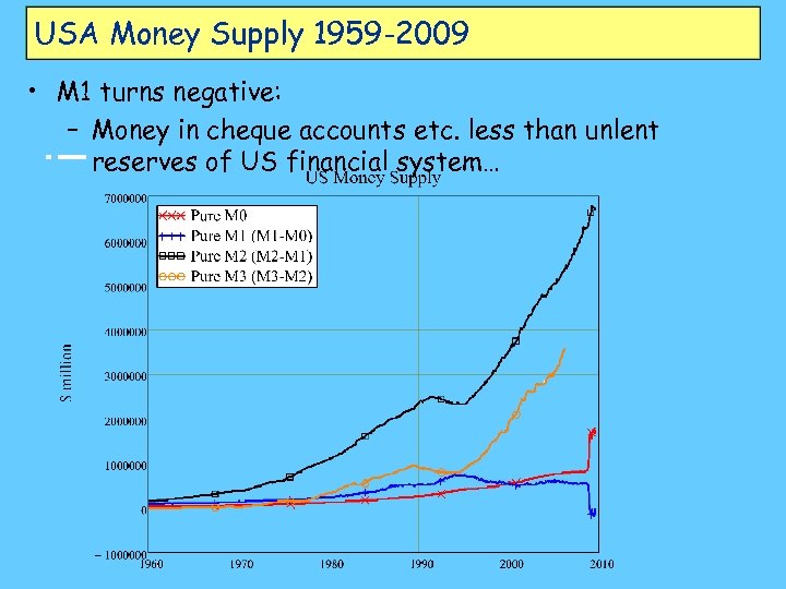
USA Money Supply 1959 -2009 • M 1 turns negative: – Money in cheque accounts etc. less than unlent reserves of US financial system…
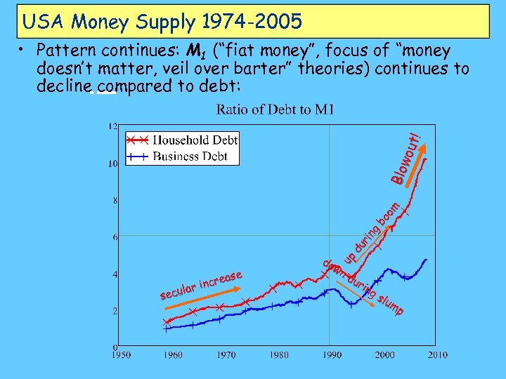
USA Money Supply 1974 -2005 du rin g bo om Blo wou t! • Pattern continues: M 1 (“fiat money”, focus of “money doesn’t matter, veil over barter” theories) continues to decline compared to debt: up do wn du rin g ase incre lar secu slu mp
Theory of endogenous money… • What does it mean to say money “endogenous”? • Strongest proponent of endogenous money is Basil Moore – US Post Keynesian economist – Criticised IS-LM model of money – Argued that Central Bank had to “accommodate” demands for liquidity of commercial banking system – Focused on mechanics of loans for large corporations • “Lines of credit” – Negotiated guaranteed access to credit for major companies with major banks – Mainly used to finance rapid changes in input costs without needing to go “cap in hand” to the bank…
Moore on endogeneity • “Changes in wages and employment largely determine the demand for bank loans, which in turn determine the rate of growth of the money stock. • Central banks have no alternative but to accept this course of events, their only option being to vary the short-term rate of interest at which they supply liquidity to the banking system on demand. • Commercial banks are now in a position to supply whatever volume of credit to the economy that their borrowers demand. ” (Moore [1] : 3 -4) • In a nutshell – The supply of money & credit is determined by the demand for money & credit. There is no independent supply curve as in standard micro theory – All the state can do is affect the price of credit (the interest rate).
Moore on endogeneity • Conventional economic theory springs from the facts that – Once, money was gold and silver coin – Today, bank notes are state-issued legal tender • Conventional theory treats the latter as just a variant of the former • Endogenous money theorists look instead at the invention of credit, when negotiable notes were first issued by private banks: – “The crucial innovation was the finding that a banking house of sufficient repute could dispense with the issue of [gold and silver] coin and instead issue its own instruments of indebtedness. The payability of bank IOUs to the bearer rather than to a named individual made them widely usable as a means of payment. ” (4)
Moore on endogeneity • Thus there is an essential difference between commodity or fiat money and credit money, but this is missed by conventional theory: – “modern monetary theory has inherited an approach to money that was more appropriate in a world where money was a commodity … without fully recognising the fundamental differences between commodity and credit money. ” (5) – The supply of commodity money is clearly limited by • new output of gold and silver • Plus accumulated saleable or hoardable stocks – Monetarist/neoclassical views ascribe the same to modern credit money:
Moore on endogeneity • In the quantity theory relation MV=PT, there is an assumption that – “is something so elementary that it is almost never discussed, reflectively considered, or even noticed: the assumption that there exists an independent supply function of money. ” (7) – This is feasible in a solely commodity or fiat money system. With a system in which money is “commodities … or … fiat debt of the government, it is easy to envision an independent supply of money function, conceptually distinct from the demand for money function. ” (7 -8) – But in a credit money system, the supply of credit adjusts to the demands of the financial and productive systems.
![Moore on endogeneity • One essential difference between commodity [gold/silver] or fiat [coins and Moore on endogeneity • One essential difference between commodity [gold/silver] or fiat [coins and](https://present5.com/presentation/ec1f5a11fc7c5816ef88bef0605f31b6/image-57.jpg)
Moore on endogeneity • One essential difference between commodity [gold/silver] or fiat [coins and notes] money and credit money is – “Because commodity money is a material thing rather than a financial claim, it is an asset to its holder but a liability to no-one. Thus, the quantity of commodity money in existence denotes nothing about the outstanding volume of credit. ” (13) – On the other hand, “Since the supply of credit money is furnished by the extension of credit [and hence debt], the supply schedule is no longer independent of debt demand… the stock of bank money is completely determined by borrowers’ demands for credit. ” (13 -14) – So what’s wrong with the quantity theory equation?
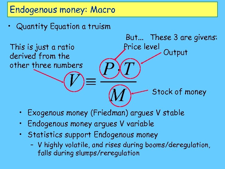
Endogenous money: Macro • Quantity Equation a truism This is just a ratio derived from the other three numbers But. . . These 3 are givens: Price level Output Stock of money • Exogenous money (Friedman) argues V stable • Endogenous money argues V variable • Statistics support Endogenous money – V highly volatile, and rises during booms/deregulation, falls during slumps/reregulation
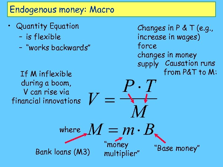
Endogenous money: Macro • Quantity Equation – is flexible – “works backwards” If M inflexible during a boom, V can rise via financial innovations Changes in P & T (e. g. , increase in wages) force changes in money supply Causation runs from P&T to M: where Bank loans (M 3) “money multiplier” “Base money”
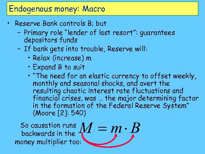
Endogenous money: Macro • Reserve Bank controls B; but – Primary role “lender of last resort”: guarantees depositors funds – If bank gets into trouble, Reserve will: • Relax (increase) m • Expand B to suit • “The need for an elastic currency to offset weekly, monthly and seasonal shocks, and avert the resulting chaotic interest rate fluctuations and financial crises, was … the major determining factor in the formation of the Federal Reserve System” (Moore [2]: 540) So causation runs backwards in the money multiplier too:
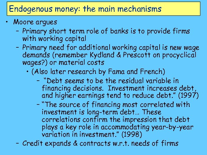
Endogenous money: the main mechanisms • Moore argues – Primary short term role of banks is to provide firms with working capital – Primary need for additional working capital is new wage demands (remember Kydland & Prescott on procyclical wages? ) or material costs • (Also later research by Fama and French) – “Debt seems to be the residual variable in financing decisions. Investment increases debt, and higher earnings tend to reduce debt. ” (1997) – “The source of financing most correlated with investment is long-term debt… These correlations confirm the impression that debt plays a key role in accommodating year-by-year variation in investment. ” (1998) – Credit expands & contracts w. r. t. needs of firms
Endogenous money: the main mechanisms • Firms face new wage/material cost/investment demand • Firms extend lines of credit with banks for working capital/investment finance shortfalls • Increased loans lead to increased deposits by recipients of expenditure – New deposits are created after the loans, but balance the new indebtedness • Central bank need to underwrite liquidity ensures changes to base/money multiplier (itself no longer monitored) accommodate additional loans • Causation thus works – From P and T to M (with volatile “V”) – From M to m and B
Endogenous money: initial consequences • The money supply is determined by the demands of the commercial sector, not by the government • It can therefore expand contract regardless of government policy • Credit money carries with it debt obligations (whereas fiat or commodity money does not), therefore debt dynamics are an important part of the monetary system • Financial behaviour of commercial sector is thus a crucial part of the economic system. • “Endogenous money” prima facie persuasive… – But some controversies in endogenous money…
ec1f5a11fc7c5816ef88bef0605f31b6.ppt