51430b84e6cb2db1d80f7535b73b43be.ppt
- Количество слайдов: 49

Beat the Mean Bandit ICML 2011 Yisong Yue Carnegie Mellon University Joint work with Thorsten Joachims (Cornell University)
Optimizing Information Retrieval Systems • Increasingly reliant on user feedback – E. g. , clicks on search results • Online learning is a popular modeling tool – Especially partial-information (bandit) settings • Our focus: learning from relative preferences – Motivated by recent work on interleaved retrievaluation (example following)
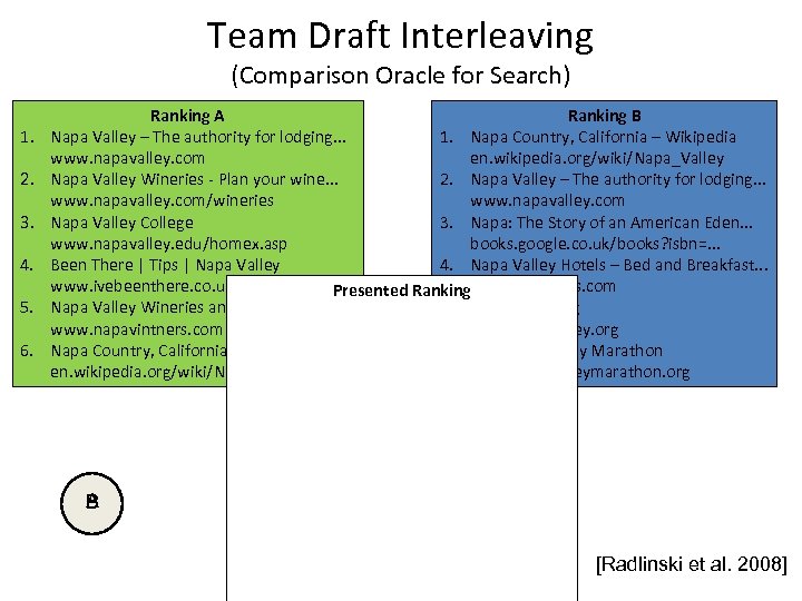
Team Draft Interleaving (Comparison Oracle for Search) 1. 2. 3. 4. 5. 6. Ranking A Ranking B Napa Valley – The authority for lodging. . . 1. Napa Country, California – Wikipedia www. napavalley. com en. wikipedia. org/wiki/Napa_Valley Napa Valley Wineries - Plan your wine. . . 2. Napa Valley – The authority for lodging. . . www. napavalley. com/wineries www. napavalley. com Napa Valley College 3. Napa: The Story of an American Eden. . . www. napavalley. edu/homex. asp books. google. co. uk/books? isbn=. . . Been There | Tips | Napa Valley 4. Napa Valley Hotels – Bed and Breakfast. . . www. ivebeenthere. co. uk/tips/16681 Presented Rankingwww. napalinks. com Napa Valley Wineries and 1. Napa Valley – The authority for lodging. . . Wine 5. Napa. Valley. org www. napavintners. com www. napavalley. org www. napavalley. com Napa Country, California – Wikipedia 2. Napa Country, California 6. Wikipedia Valley Marathon – The Napa en. wikipedia. org/wiki/Napa_Valley www. napavalleymarathon. org en. wikipedia. org/wiki/Napa_Valley 3. Napa: The Story of an American Eden. . . books. google. co. uk/books? isbn=. . . 4. Napa Valley Wineries – Plan your wine. . . www. napavalley. com/wineries 5. Napa Valley Hotels – Bed and Breakfast. . . A B www. napalinks. com 6. Napa Balley College www. napavalley. edu/homex. asp [Radlinski et al. 2008] 7 Napa. Valley. org www. napavalley. org
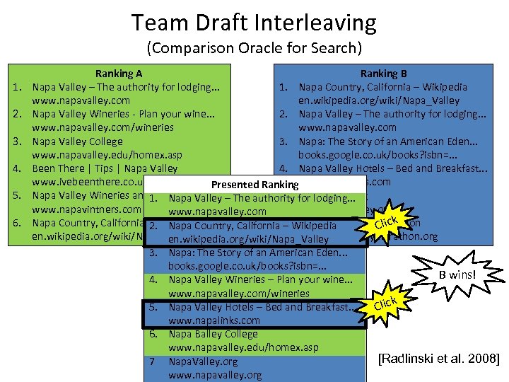
Team Draft Interleaving (Comparison Oracle for Search) 1. 2. 3. 4. 5. 6. Ranking A Ranking B Napa Valley – The authority for lodging. . . 1. Napa Country, California – Wikipedia www. napavalley. com en. wikipedia. org/wiki/Napa_Valley Napa Valley Wineries - Plan your wine. . . 2. Napa Valley – The authority for lodging. . . www. napavalley. com/wineries www. napavalley. com Napa Valley College 3. Napa: The Story of an American Eden. . . www. napavalley. edu/homex. asp books. google. co. uk/books? isbn=. . . Been There | Tips | Napa Valley 4. Napa Valley Hotels – Bed and Breakfast. . . www. ivebeenthere. co. uk/tips/16681 Presented Rankingwww. napalinks. com Napa Valley Wineries and 1. Napa Valley – The authority for lodging. . . Wine 5. Napa. Valley. org www. napavintners. com www. napavalley. org www. napavalley. com Napa Country, California – Wikipedia 2. Napa Country, California 6. Wikipedia Valley Marathon – The Napa Click en. wikipedia. org/wiki/Napa_Valley www. napavalleymarathon. org en. wikipedia. org/wiki/Napa_Valley 3. Napa: The Story of an American Eden. . . books. google. co. uk/books? isbn=. . . B wins! 4. Napa Valley Wineries – Plan your wine. . . www. napavalley. com/wineries 5. Napa Valley Hotels – Bed and Breakfast. . . Click www. napalinks. com 6. Napa Balley College www. napavalley. edu/homex. asp [Radlinski et al. 2008] 7 Napa. Valley. org www. napavalley. org
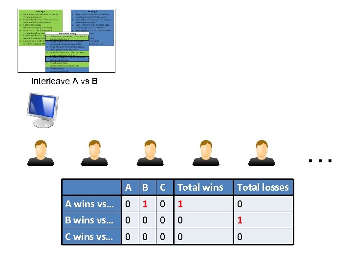
Interleave A vs B … A B C Total wins Total losses A wins vs… 0 1 0 B wins vs… 0 0 1 C wins vs… 0 0 0
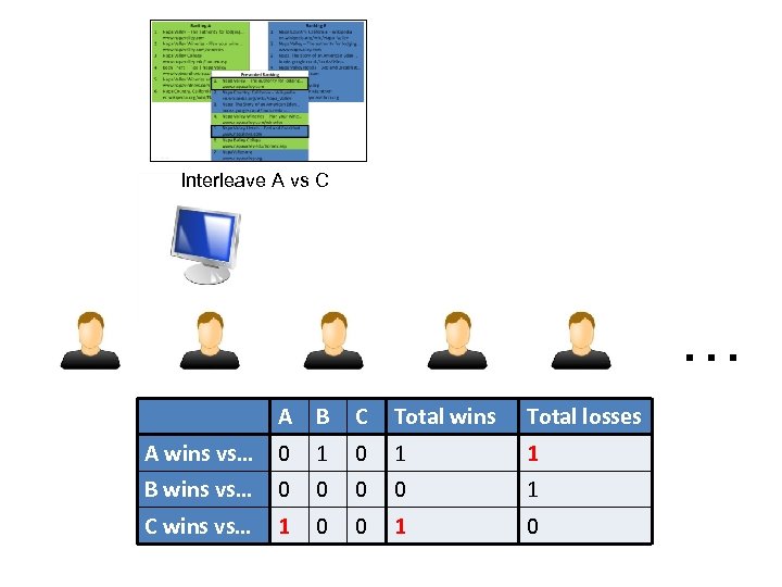
Interleave A vs C … A B C Total wins Total losses A wins vs… 0 1 1 B wins vs… 0 0 1 C wins vs… 1 0 0 1 0
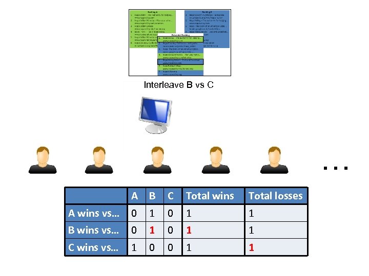
Interleave B vs C … A B C Total wins Total losses A wins vs… 0 1 1 B wins vs… 0 1 1 C wins vs… 1 0 0 1 1
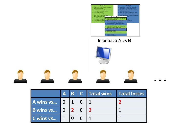
Interleave A vs B … A B C Total wins Total losses A wins vs… 0 1 2 B wins vs… 0 2 1 C wins vs… 1 0 0 1 1
![Outline • Learning Formulation – Dueling Bandits Problem [Yue et al. 2009] • Modeling Outline • Learning Formulation – Dueling Bandits Problem [Yue et al. 2009] • Modeling](https://present5.com/presentation/51430b84e6cb2db1d80f7535b73b43be/image-9.jpg)
Outline • Learning Formulation – Dueling Bandits Problem [Yue et al. 2009] • Modeling transitivity violation – E. g. , (A >> B) AND (B >> C) IMPLIES (A >> C) ? ? – Not done in previous work
![Outline • Learning Formulation – Dueling Bandits Problem [Yue et al. 2009] • Modeling Outline • Learning Formulation – Dueling Bandits Problem [Yue et al. 2009] • Modeling](https://present5.com/presentation/51430b84e6cb2db1d80f7535b73b43be/image-10.jpg)
Outline • Learning Formulation – Dueling Bandits Problem [Yue et al. 2009] • Modeling transitivity violation – E. g. , (A >> B) AND (B >> C) IMPLIES (A >> C) ? ? – Not done in previous work • Algorithm: Beat-the-Mean • Empirical Validation
Dueling Bandits Problem • Given K bandits b 1, …, b. K • Each iteration: compare (duel) two bandits – E. g. , interleaving two retrieval functions [Yue et al. 2009]
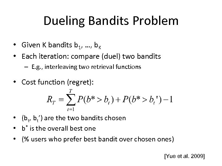
Dueling Bandits Problem • Given K bandits b 1, …, b. K • Each iteration: compare (duel) two bandits – E. g. , interleaving two retrieval functions • Cost function (regret): • (bt, bt’) are the two bandits chosen • b* is the overall best one • (% users who prefer best bandit over chosen ones) [Yue et al. 2009]
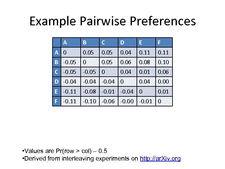
Example Pairwise Preferences A B C D E F A 0 0. 05 0. 04 0. 11 B -0. 05 0. 06 0. 08 0. 10 C -0. 05 0 0. 04 0. 01 0. 06 D -0. 04 0 0. 04 0. 00 E -0. 11 -0. 08 -0. 01 -0. 04 0 F -0. 11 -0. 10 -0. 06 -0. 00 -0. 01 0 0. 01 • Values are Pr(row > col) – 0. 5 • Derived from interleaving experiments on http: //ar. Xiv. org
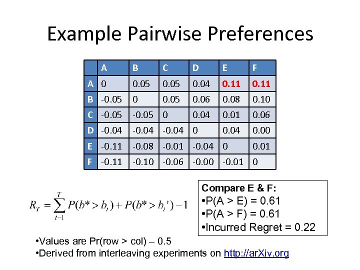
Example Pairwise Preferences A B C D E F A 0 0. 05 0. 04 0. 11 B -0. 05 0. 06 0. 08 0. 10 C -0. 05 0 0. 04 0. 01 0. 06 D -0. 04 0 0. 04 0. 00 E -0. 11 -0. 08 -0. 01 -0. 04 0 F -0. 11 -0. 10 -0. 06 -0. 00 -0. 01 0 0. 01 Compare E & F: • P(A > E) = 0. 61 • P(A > F) = 0. 61 • Incurred Regret = 0. 22 • Values are Pr(row > col) – 0. 5 • Derived from interleaving experiments on http: //ar. Xiv. org
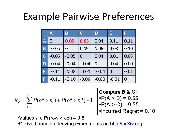
Example Pairwise Preferences A B C D E F A 0 0. 05 0. 04 0. 11 B -0. 05 0. 06 0. 08 0. 10 C -0. 05 0 0. 04 0. 01 0. 06 D -0. 04 0 0. 04 0. 00 E -0. 11 -0. 08 -0. 01 -0. 04 0 F -0. 11 -0. 10 -0. 06 -0. 00 -0. 01 0 0. 01 Compare B & C: • P(A > B) = 0. 55 • P(A > C) = 0. 55 • Incurred Regret = 0. 10 • Values are Pr(row > col) – 0. 5 • Derived from interleaving experiments on http: //ar. Xiv. org
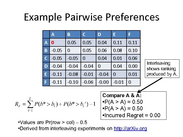
Example Pairwise Preferences A B C D E F A 0 0. 05 0. 04 0. 11 B -0. 05 0. 06 0. 08 0. 10 C -0. 05 0 0. 04 0. 01 0. 06 D -0. 04 0 0. 04 0. 00 E -0. 11 -0. 08 -0. 01 -0. 04 0 F -0. 11 -0. 10 -0. 06 -0. 00 -0. 01 0 0. 01 Interleaving shows ranking produced by A. Compare A & A: • P(A > A) = 0. 50 • Incurred Regret = 0. 00 • Values are Pr(row > col) – 0. 5 • Derived from interleaving experiments on http: //ar. Xiv. org
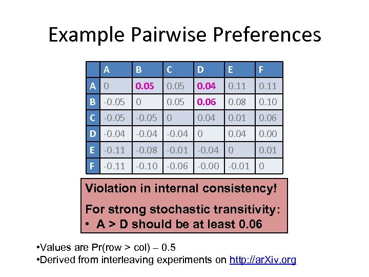
Example Pairwise Preferences A B C D E F A 0 0. 05 0. 04 0. 11 B -0. 05 0. 06 0. 08 0. 10 C -0. 05 0 0. 04 0. 01 0. 06 D -0. 04 0 0. 04 0. 00 E -0. 11 -0. 08 -0. 01 -0. 04 0 F -0. 11 -0. 10 -0. 06 -0. 00 -0. 01 0 0. 01 Violation in internal consistency! For strong stochastic transitivity: • A > D should be at least 0. 06 • Values are Pr(row > col) – 0. 5 • Derived from interleaving experiments on http: //ar. Xiv. org
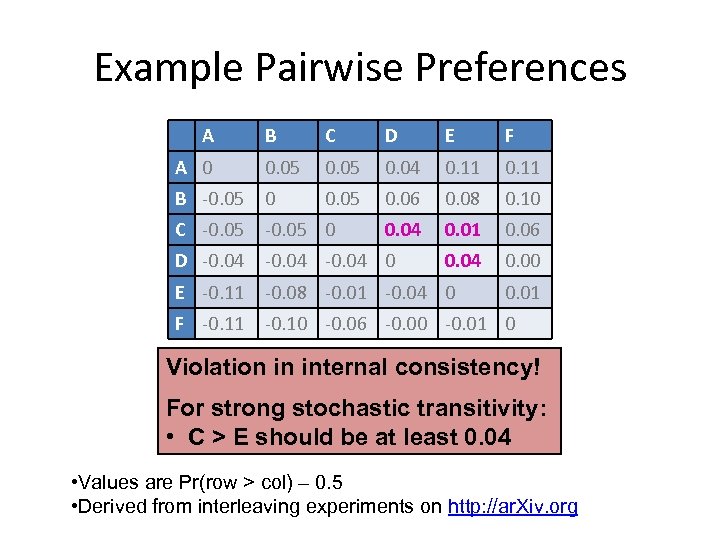
Example Pairwise Preferences A B C D E F A 0 0. 05 0. 04 0. 11 B -0. 05 0. 06 0. 08 0. 10 C -0. 05 0 0. 04 0. 01 0. 06 D -0. 04 0 0. 04 0. 00 E -0. 11 -0. 08 -0. 01 -0. 04 0 F -0. 11 -0. 10 -0. 06 -0. 00 -0. 01 0 0. 01 Violation in internal consistency! For strong stochastic transitivity: • C > E should be at least 0. 04 • Values are Pr(row > col) – 0. 5 • Derived from interleaving experiments on http: //ar. Xiv. org
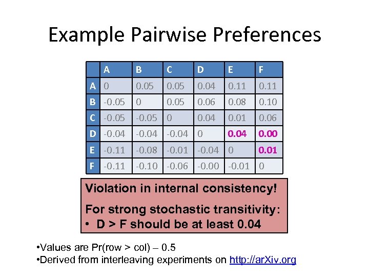
Example Pairwise Preferences A B C D E F A 0 0. 05 0. 04 0. 11 B -0. 05 0. 06 0. 08 0. 10 C -0. 05 0 0. 04 0. 01 0. 06 D -0. 04 0 0. 04 0. 00 E -0. 11 -0. 08 -0. 01 -0. 04 0 F -0. 11 -0. 10 -0. 06 -0. 00 -0. 01 0 0. 01 Violation in internal consistency! For strong stochastic transitivity: • D > F should be at least 0. 04 • Values are Pr(row > col) – 0. 5 • Derived from interleaving experiments on http: //ar. Xiv. org
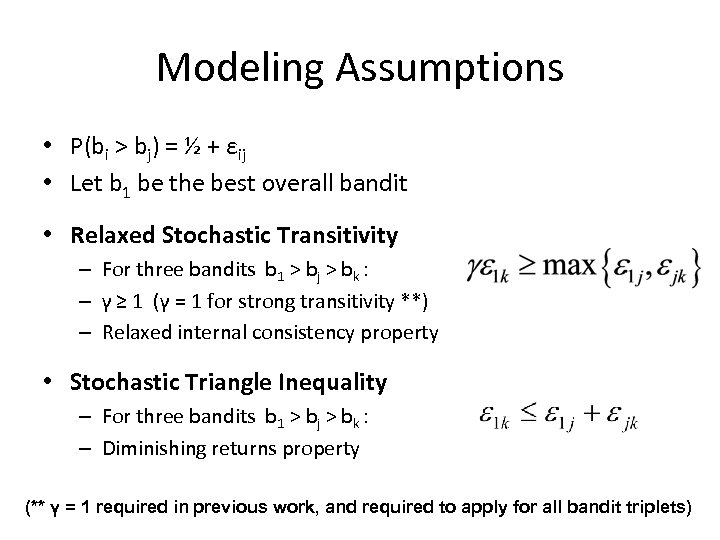
Modeling Assumptions • P(bi > bj) = ½ + εij • Let b 1 be the best overall bandit • Relaxed Stochastic Transitivity – For three bandits b 1 > bj > bk : – γ ≥ 1 (γ = 1 for strong transitivity **) – Relaxed internal consistency property • Stochastic Triangle Inequality – For three bandits b 1 > bj > bk : – Diminishing returns property (** γ = 1 required in previous work, and required to apply for all bandit triplets)
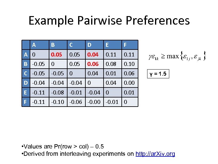
Example Pairwise Preferences A B C D E F A 0 0. 05 0. 04 0. 11 B -0. 05 0. 06 0. 08 0. 10 C -0. 05 0 0. 04 0. 01 0. 06 D -0. 04 0 0. 04 0. 00 E -0. 11 -0. 08 -0. 01 -0. 04 0 F -0. 11 -0. 10 -0. 06 -0. 00 -0. 01 0 γ = 1. 5 0. 01 • Values are Pr(row > col) – 0. 5 • Derived from interleaving experiments on http: //ar. Xiv. org
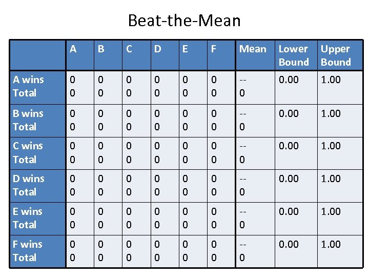
Beat-the-Mean A B C D E F Mean Lower Bound Upper Bound A wins Total 0 0 0 -0 0. 00 1. 00 B wins Total 0 0 0 -0 0. 00 1. 00 C wins Total 0 0 0 -0 0. 00 1. 00 D wins Total 0 0 0 -0 0. 00 1. 00 E wins Total 0 0 0 -0 0. 00 1. 00 F wins Total 0 0 0 -0 0. 00 1. 00
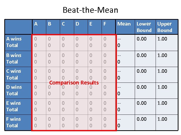
Beat-the-Mean A B C D E F Mean Lower Bound Upper Bound A wins Total 0 0 0 -0 0. 00 1. 00 B wins Total 0 0 0 -0 0. 00 1. 00 C wins Total 0 0 0 -0 0. 00 1. 00 D wins Total 0 0 0 -0 0. 00 1. 00 E wins Total 0 0 0 -0 0. 00 1. 00 F wins Total 0 0 0 -0 0. 00 1. 00 Comparison Results
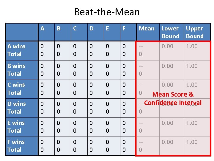
Beat-the-Mean A B C D E F Mean Lower Bound Upper Bound A wins Total 0 0 0 -0 0. 00 1. 00 B wins Total 0 0 0 -0 0. 00 1. 00 C wins Total 0 0 0 -0 0. 00 1. 00 D wins Total 0 0 0 0 E wins Total 0 0 0 -0 0. 00 1. 00 F wins Total 0 0 0 -0 0. 00 1. 00 Mean Score & -- Confidence Interval 0. 00 1. 00
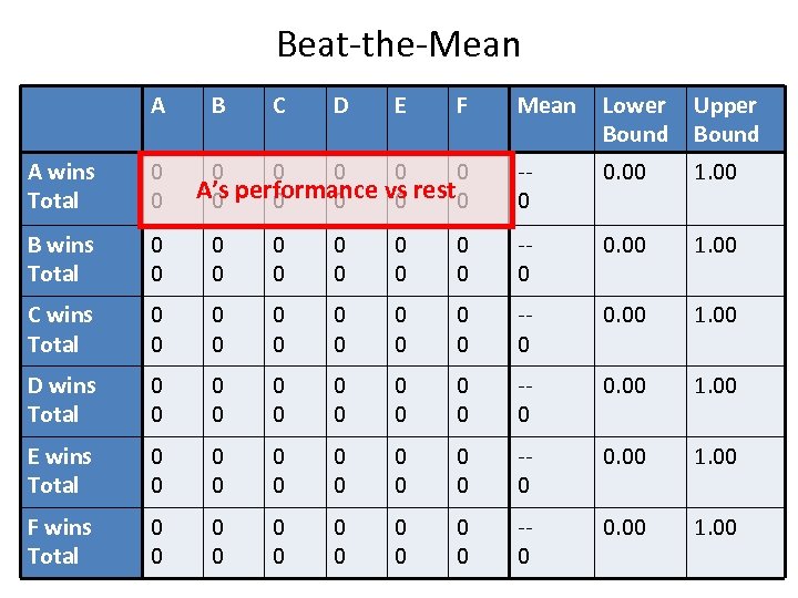
Beat-the-Mean A B C D E F 0 0 0 A’s performance vs rest 0 0 0 Mean Lower Bound Upper Bound -0 0. 00 1. 00 A wins Total 0 0 B wins Total 0 0 0 -0 0. 00 1. 00 C wins Total 0 0 0 -0 0. 00 1. 00 D wins Total 0 0 0 -0 0. 00 1. 00 E wins Total 0 0 0 -0 0. 00 1. 00 F wins Total 0 0 0 -0 0. 00 1. 00
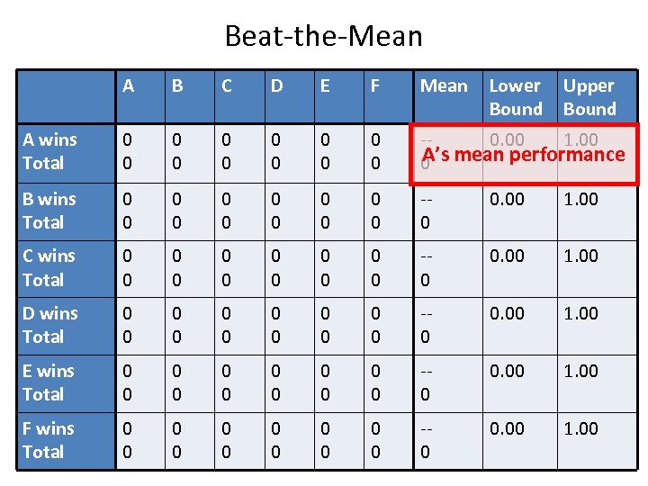
Beat-the-Mean A B C D E F Mean Lower Bound Upper Bound A wins Total 0 0 0 -0. 00 1. 00 A’s 0 mean performance B wins Total 0 0 0 -0 0. 00 1. 00 C wins Total 0 0 0 -0 0. 00 1. 00 D wins Total 0 0 0 -0 0. 00 1. 00 E wins Total 0 0 0 -0 0. 00 1. 00 F wins Total 0 0 0 -0 0. 00 1. 00
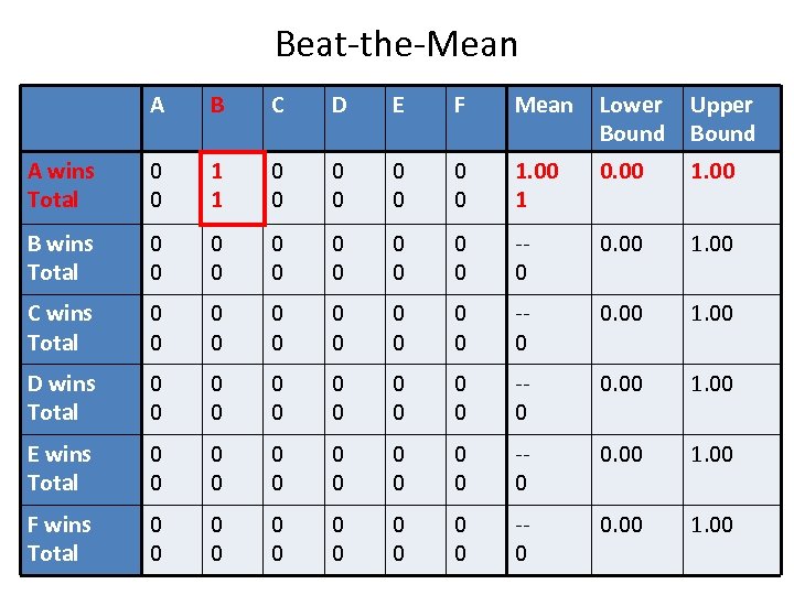
Beat-the-Mean A B C D E F Mean Lower Bound Upper Bound A wins Total 0 0 1 1 0 0 0 0 1. 00 1 0. 00 1. 00 B wins Total 0 0 0 -0 0. 00 1. 00 C wins Total 0 0 0 -0 0. 00 1. 00 D wins Total 0 0 0 -0 0. 00 1. 00 E wins Total 0 0 0 -0 0. 00 1. 00 F wins Total 0 0 0 -0 0. 00 1. 00
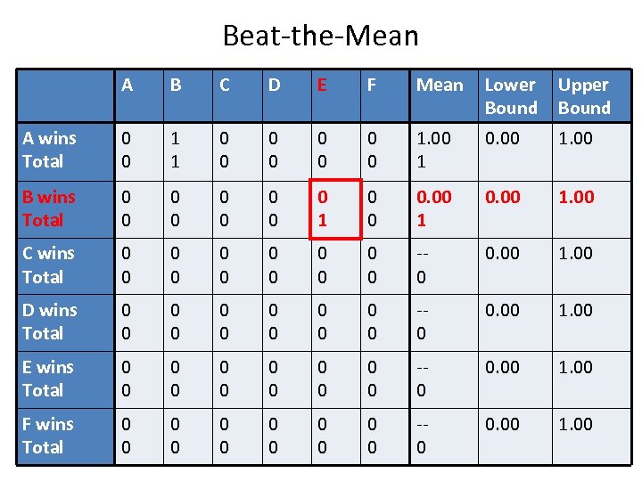
Beat-the-Mean A B C D E F Mean Lower Bound Upper Bound A wins Total 0 0 1 1 0 0 0 0 1. 00 1 0. 00 1. 00 B wins Total 0 0 0 0 0 1 0 0 0. 00 1. 00 C wins Total 0 0 0 -0 0. 00 1. 00 D wins Total 0 0 0 -0 0. 00 1. 00 E wins Total 0 0 0 -0 0. 00 1. 00 F wins Total 0 0 0 -0 0. 00 1. 00
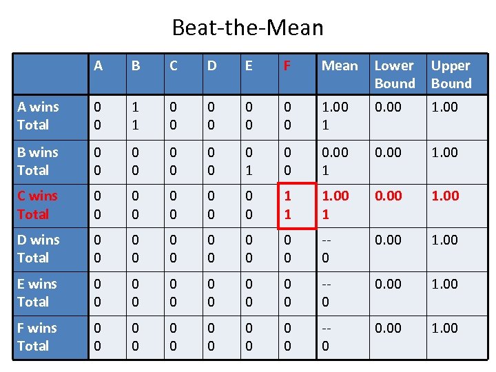
Beat-the-Mean A B C D E F Mean Lower Bound Upper Bound A wins Total 0 0 1 1 0 0 0 0 1. 00 1 0. 00 1. 00 B wins Total 0 0 0 0 0 1 0 0 0. 00 1. 00 C wins Total 0 0 0 0 0 1 1 1. 00 1 0. 00 1. 00 D wins Total 0 0 0 -0 0. 00 1. 00 E wins Total 0 0 0 -0 0. 00 1. 00 F wins Total 0 0 0 -0 0. 00 1. 00
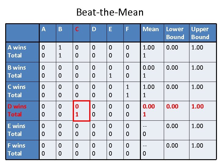
Beat-the-Mean A B C D E F Mean Lower Bound Upper Bound A wins Total 0 0 1 1 0 0 0 0 1. 00 1 0. 00 1. 00 B wins Total 0 0 0 0 0 1 0 0 0. 00 1. 00 C wins Total 0 0 0 0 0 1 1 1. 00 1 0. 00 1. 00 D wins Total 0 0 0 1 0 0 0 0. 00 1. 00 E wins Total 0 0 0 -0 0. 00 1. 00 F wins Total 0 0 0 -0 0. 00 1. 00
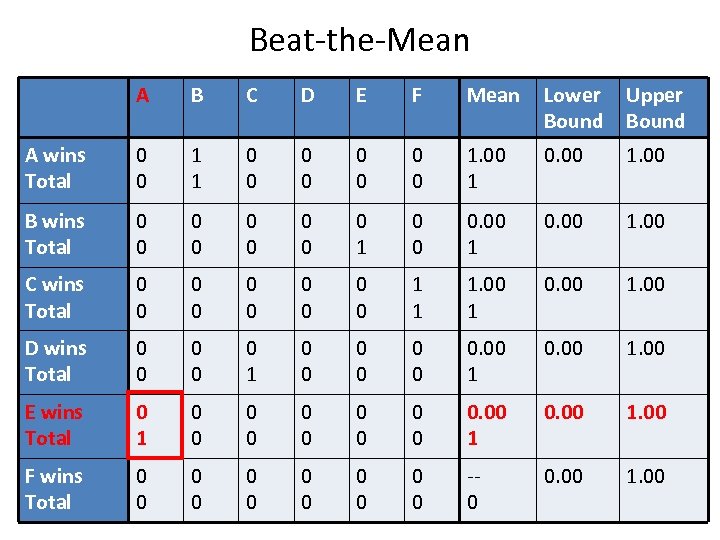
Beat-the-Mean A B C D E F Mean Lower Bound Upper Bound A wins Total 0 0 1 1 0 0 0 0 1. 00 1 0. 00 1. 00 B wins Total 0 0 0 0 0 1 0 0 0. 00 1. 00 C wins Total 0 0 0 0 0 1 1 1. 00 1 0. 00 1. 00 D wins Total 0 0 0 1 0 0 0 0. 00 1. 00 E wins Total 0 1 0 0 0. 00 1. 00 F wins Total 0 0 0 -0 0. 00 1. 00
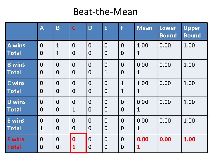
Beat-the-Mean A B C D E F Mean Lower Bound Upper Bound A wins Total 0 0 1 1 0 0 0 0 1. 00 1 0. 00 1. 00 B wins Total 0 0 0 0 0 1 0 0 0. 00 1. 00 C wins Total 0 0 0 0 0 1 1 1. 00 1 0. 00 1. 00 D wins Total 0 0 0 1 0 0 0 0. 00 1. 00 E wins Total 0 1 0 0 0. 00 1. 00 F wins Total 0 0 0 1 0 0 0 0. 00 1. 00
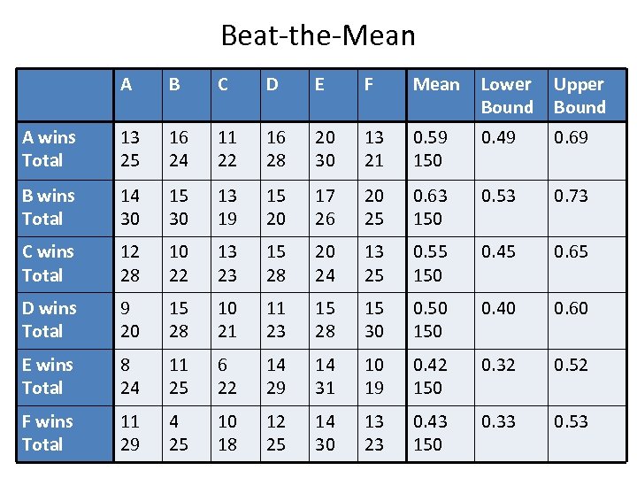
Beat-the-Mean A B C D E F Mean Lower Bound Upper Bound A wins Total 13 25 16 24 11 22 16 28 20 30 13 21 0. 59 150 0. 49 0. 69 B wins Total 14 30 15 30 13 19 15 20 17 26 20 25 0. 63 150 0. 53 0. 73 C wins Total 12 28 10 22 13 23 15 28 20 24 13 25 0. 55 150 0. 45 0. 65 D wins Total 9 20 15 28 10 21 11 23 15 28 15 30 0. 50 150 0. 40 0. 60 E wins Total 8 24 11 25 6 22 14 29 14 31 10 19 0. 42 150 0. 32 0. 52 F wins Total 11 29 4 25 10 18 12 25 14 30 13 23 0. 43 150 0. 33 0. 53
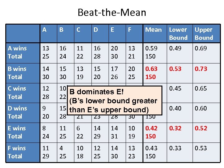
Beat-the-Mean A B C D E F Mean Lower Bound Upper Bound A wins Total 13 25 16 24 11 22 16 28 20 30 13 21 0. 59 150 0. 49 0. 69 B wins Total 14 30 15 30 13 19 15 20 17 26 20 25 0. 63 150 0. 53 0. 73 C wins Total 12 28 10 13 15 20 13 B dominates E! 22 23 28 24 25 0. 55 150 0. 45 0. 65 D wins Total 9 20 0. 40 0. 60 E wins Total F wins Total (B’s lower bound greater 15 than E’s upper bound) 10 11 15 15 0. 50 28 21 23 28 30 150 8 24 11 25 6 22 14 29 14 31 10 19 0. 42 150 0. 32 0. 52 11 29 4 25 10 18 12 25 14 30 13 23 0. 43 150 0. 33 0. 53
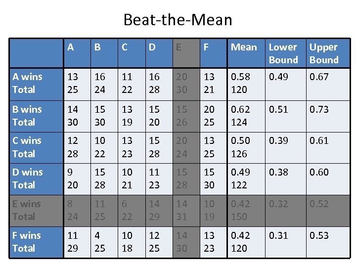
Beat-the-Mean A B C D E F Mean Lower Bound Upper Bound A wins Total 13 25 16 24 11 22 16 28 20 30 13 21 0. 58 120 0. 49 0. 67 B wins Total 14 30 15 30 13 19 15 20 15 26 20 25 0. 62 124 0. 51 0. 73 C wins Total 12 28 10 22 13 23 15 28 20 24 13 25 0. 50 126 0. 39 0. 61 D wins Total 9 20 15 28 10 21 11 23 15 28 15 30 0. 49 122 0. 38 0. 60 E wins Total 8 24 11 25 6 22 14 29 14 31 10 19 0. 42 150 0. 32 0. 52 F wins Total 11 29 4 25 10 18 12 25 14 30 13 23 0. 42 120 0. 31 0. 53
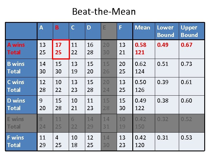
Beat-the-Mean A B C D E F Mean Lower Bound Upper Bound A wins Total 13 25 17 25 11 22 16 28 20 30 13 21 0. 58 121 0. 49 0. 67 B wins Total 14 30 15 30 13 19 15 20 15 26 20 25 0. 62 124 0. 51 0. 73 C wins Total 12 28 10 22 13 23 15 28 20 24 13 25 0. 50 126 0. 39 0. 61 D wins Total 9 20 15 28 10 21 11 23 15 28 15 30 0. 49 122 0. 38 0. 60 E wins Total 8 24 11 25 6 22 14 29 14 31 10 19 0. 42 150 0. 32 0. 52 F wins Total 11 29 4 25 10 18 12 25 14 30 13 23 0. 42 120 0. 31 0. 53
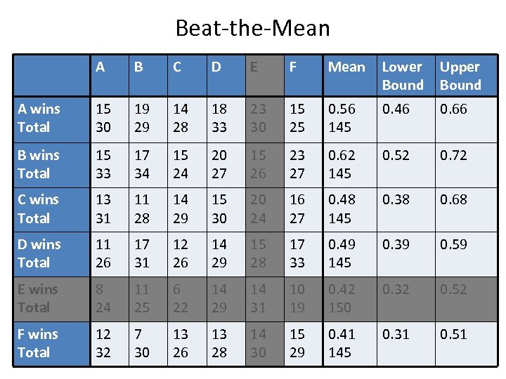
Beat-the-Mean A B C D E F Mean Lower Bound Upper Bound A wins Total 15 30 19 29 14 28 18 33 23 30 15 25 0. 56 145 0. 46 0. 66 B wins Total 15 33 17 34 15 24 20 27 15 26 23 27 0. 62 145 0. 52 0. 72 C wins Total 13 31 11 28 14 29 15 30 20 24 16 27 0. 48 145 0. 38 0. 68 D wins Total 11 26 17 31 12 26 14 29 15 28 17 33 0. 49 145 0. 39 0. 59 E wins Total 8 24 11 25 6 22 14 29 14 31 10 19 0. 42 150 0. 32 0. 52 F wins Total 12 32 7 30 13 26 13 28 14 30 15 29 0. 41 145 0. 31 0. 51
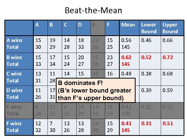
Beat-the-Mean A B C D E F Mean Lower Bound Upper Bound A wins Total 15 30 19 29 14 28 18 33 23 30 15 25 0. 56 145 0. 46 0. 66 B wins Total 15 33 17 34 15 24 20 27 15 26 23 27 0. 62 145 0. 52 0. 72 C wins Total 13 31 0. 38 0. 68 D wins Total 11 26 11 14 15 20 16 0. 48 28 B 29 30 24 27 145 dominates F! 17 (B’s lower bound greater 12 14 15 17 0. 49 31 than F’s upper bound) 26 29 28 33 145 0. 39 0. 59 E wins Total 8 24 11 25 6 22 14 29 14 31 10 19 0. 42 150 0. 32 0. 52 F wins Total 12 32 7 30 13 26 13 28 14 30 15 29 0. 41 145 0. 31 0. 51
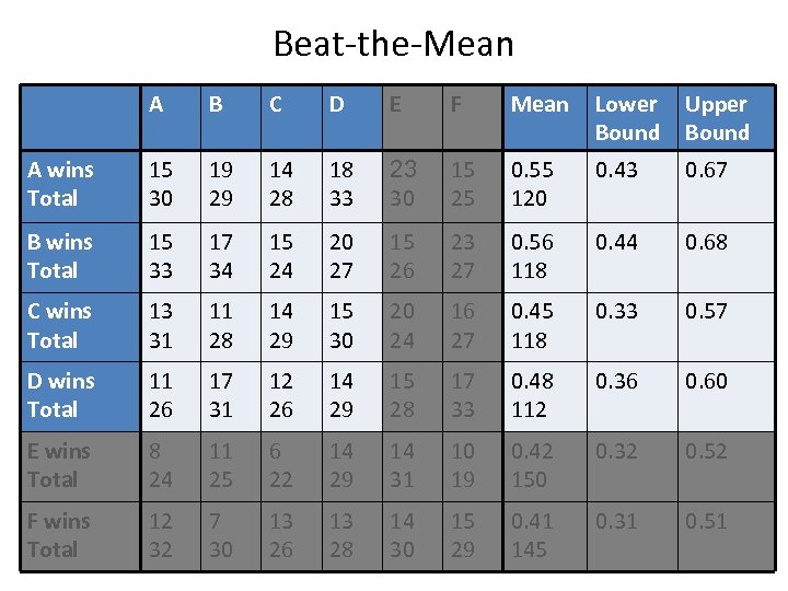
Beat-the-Mean A B C D E F Mean Lower Bound Upper Bound A wins Total 15 30 19 29 14 28 18 33 23 30 15 25 0. 55 120 0. 43 0. 67 B wins Total 15 33 17 34 15 24 20 27 15 26 23 27 0. 56 118 0. 44 0. 68 C wins Total 13 31 11 28 14 29 15 30 20 24 16 27 0. 45 118 0. 33 0. 57 D wins Total 11 26 17 31 12 26 14 29 15 28 17 33 0. 48 112 0. 36 0. 60 E wins Total 8 24 11 25 6 22 14 29 14 31 10 19 0. 42 150 0. 32 0. 52 F wins Total 12 32 7 30 13 26 13 28 14 30 15 29 0. 41 145 0. 31 0. 51
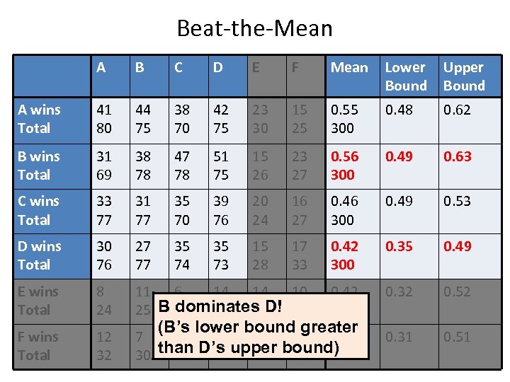
Beat-the-Mean A B C D E F Mean Lower Bound Upper Bound A wins Total 41 80 44 75 38 70 42 75 23 30 15 25 0. 55 300 0. 48 0. 62 B wins Total 31 69 38 78 47 78 51 75 15 26 23 27 0. 56 300 0. 49 0. 63 C wins Total 33 77 31 77 35 70 39 76 20 24 16 27 0. 46 300 0. 49 0. 53 D wins Total 30 76 27 77 35 74 35 73 15 28 17 33 0. 42 300 0. 35 0. 49 E wins Total 8 24 11 6 14 14 10 dominates D! 25 B 22 29 31 19 0. 42 150 0. 32 0. 52 F wins Total 12 32 7 13 13 14 15 0. 41 30 than D’s upper bound) 26 28 30 29 145 0. 31 0. 51 (B’s lower bound greater
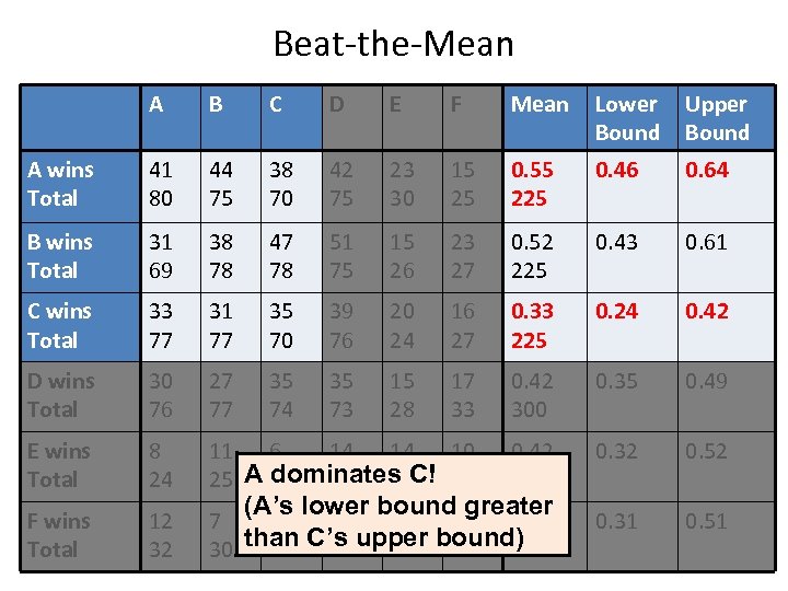
Beat-the-Mean A B C D E F Mean Lower Bound Upper Bound A wins Total 41 80 44 75 38 70 42 75 23 30 15 25 0. 55 225 0. 46 0. 64 B wins Total 31 69 38 78 47 78 51 75 15 26 23 27 0. 52 225 0. 43 0. 61 C wins Total 33 77 31 77 35 70 39 76 20 24 16 27 0. 33 225 0. 24 0. 42 D wins Total 30 76 27 77 35 74 35 73 15 28 17 33 0. 42 300 0. 35 0. 49 E wins Total 8 24 11 6 14 14 10 dominates C! 25 A 22 29 31 19 0. 42 150 0. 32 0. 52 F wins Total 12 32 7 13 13 14 15 0. 41 30 than C’s upper bound) 26 28 30 29 145 0. 31 0. 51 (A’s lower bound greater
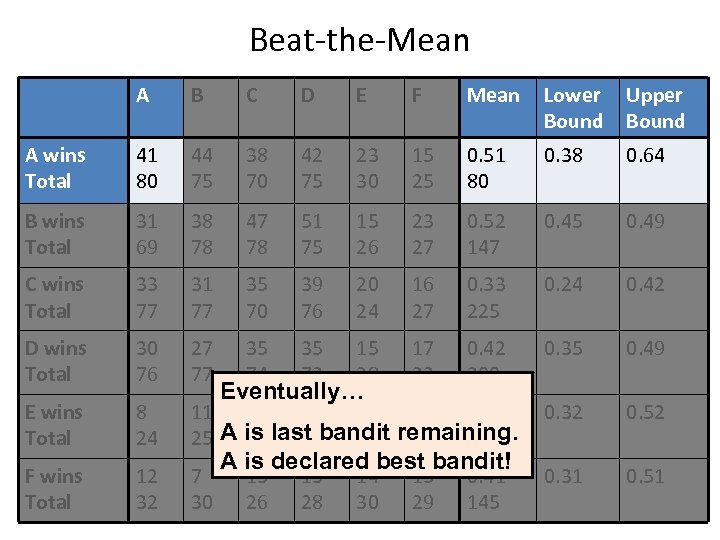
Beat-the-Mean A B C D E F Mean Lower Bound Upper Bound A wins Total 41 80 44 75 38 70 42 75 23 30 15 25 0. 51 80 0. 38 0. 64 B wins Total 31 69 38 78 47 78 51 75 15 26 23 27 0. 52 147 0. 45 0. 49 C wins Total 33 77 31 77 35 70 39 76 20 24 16 27 0. 33 225 0. 24 0. 42 D wins Total 30 76 27 77 35 74 35 73 15 28 17 33 0. 42 300 0. 35 0. 49 E wins Total 8 24 11 6 14 14 10 0. 42 25 A is last bandit remaining. 22 29 31 19 150 0. 32 0. 52 F wins Total 12 32 7 30 0. 31 0. 51 Eventually… A is declared best bandit! 13 26 13 28 14 30 15 29 0. 41 145
Regret Guarantee • Playing against mean bandit calibrates preference scores – Estimates of (active) bandits directly comparable – One estimate per active bandit = linear number of estimates
Regret Guarantee • Playing against mean bandit calibrates preference scores – Estimates of (active) bandits directly comparable – One estimate per active bandit = linear number of estimates • We can bound comparisons needed to remove worst bandit – Varies smoothly with transitivity parameter γ – High probability bound • We can bound the regret incurred by each comparison – Varies smoothly with transitivity parameter γ
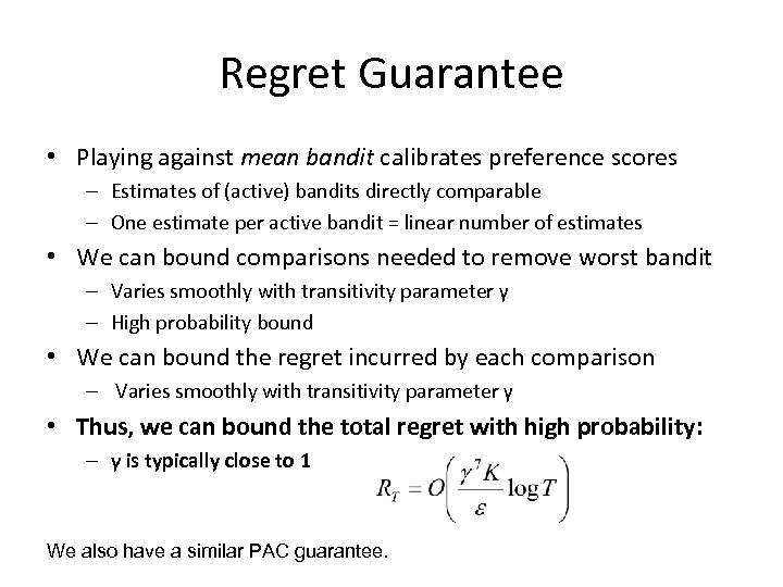
Regret Guarantee • Playing against mean bandit calibrates preference scores – Estimates of (active) bandits directly comparable – One estimate per active bandit = linear number of estimates • We can bound comparisons needed to remove worst bandit – Varies smoothly with transitivity parameter γ – High probability bound • We can bound the regret incurred by each comparison – Varies smoothly with transitivity parameter γ • Thus, we can bound the total regret with high probability: – γ is typically close to 1 We also have a similar PAC guarantee.
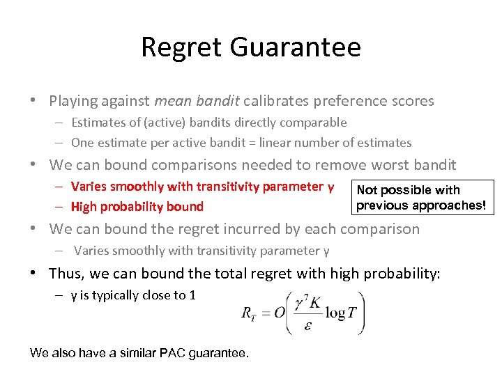
Regret Guarantee • Playing against mean bandit calibrates preference scores – Estimates of (active) bandits directly comparable – One estimate per active bandit = linear number of estimates • We can bound comparisons needed to remove worst bandit – Varies smoothly with transitivity parameter γ – High probability bound Not possible with previous approaches! • We can bound the regret incurred by each comparison – Varies smoothly with transitivity parameter γ • Thus, we can bound the total regret with high probability: – γ is typically close to 1 We also have a similar PAC guarantee.
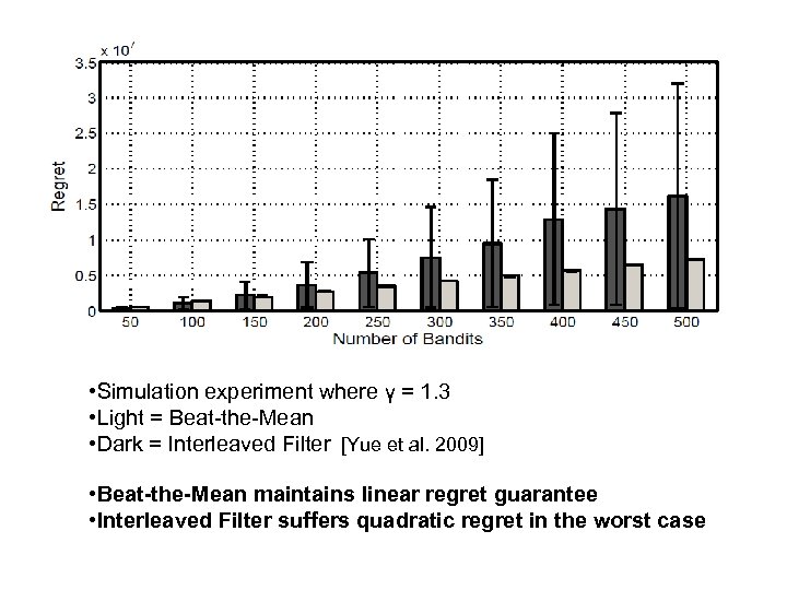
• Simulation experiment where γ = 1. 3 • Light = Beat-the-Mean • Dark = Interleaved Filter [Yue et al. 2009] • Beat-the-Mean maintains linear regret guarantee • Interleaved Filter suffers quadratic regret in the worst case
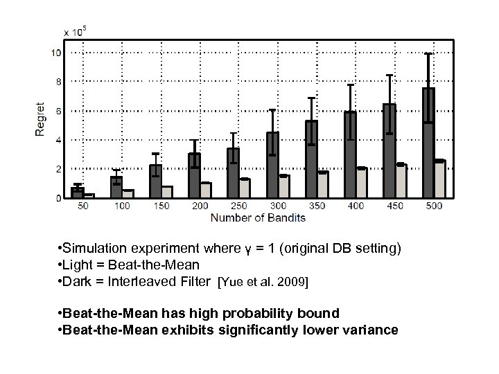
• Simulation experiment where γ = 1 (original DB setting) • Light = Beat-the-Mean • Dark = Interleaved Filter [Yue et al. 2009] • Beat-the-Mean has high probability bound • Beat-the-Mean exhibits significantly lower variance
Conclusions • Online learning approach using pairwise feedback – Well-suited for optimizing information retrieval systems from user feedback – Models violations in preference transitivity • Algorithm: Beat-the-Mean – – Regret linear in #bandits and logarithmic in #iterations Degrades smoothly with transitivity violation Stronger guarantees than previous work Empirically supported
51430b84e6cb2db1d80f7535b73b43be.ppt