394d87cc79139373840e6cb7947aaaf9.ppt
- Количество слайдов: 19
Bayesian Supplement To Freedman, Pisani, Purvis and Adhikari’s Statistics Dalene Stangl Three Parts Bayes’ Inference (Discrete) Bayes’ Inference (Continuous) GUSTO Case Study 1
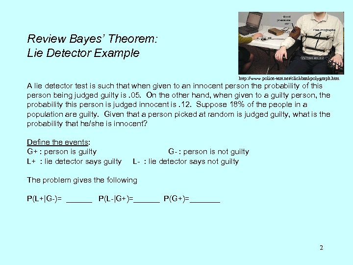
Review Bayes’ Theorem: Lie Detector Example http: //www. police-test. net/clickbankpolygraph. htm A lie detector test is such that when given to an innocent person the probability of this person being judged guilty is. 05. On the other hand, when given to a guilty person, the probability this person is judged innocent is. 12. Suppose 18% of the people in a population are guilty. Given that a person picked at random is judged guilty, what is the probability that he/she is innocent? Define the events: G+ : person is guilty G- : person is not guilty L+ : lie detector says guilty L- : lie detector says not guilty The problem gives the following P(L+|G-)= ______ P(L-|G+)=______ P(G+)=_______ 2
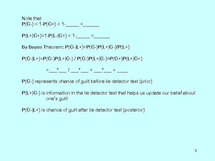
Note that P(G-) = 1 -P(G+) = 1 -_____ =______ P(L+|G+)=1 -P(L-|G+) = 1 -_____ =______ By Bayes Theorem: P(G-|L+)=P(G-)P(L+|G-)/P(L+) P(G-|L+)=P(G-)P(L+|G-) / P(G-)P(L+|G-)+P(G+)P(L+|G+) =___*___ / ___*___ + ___*___ = ____ P(G-) represents chance of guilt before lie detector test (prior) P(L+|G-) is information in the lie detector test that helps us update our belief about one’s guilt P(G-|L+) is chance of guilt after lie detector test (posterior) 3

Bayes Theorem: Big Picture P(A|B)=P(B|A)P(A) P(B) This theorem is a formalism for how we learn. P(A) is what we know about the chances of A prior to getting information from B. Then we combine our prior information with our current information, P(B|A), to come up with what we now know about the chances of A, P(A|B). P(A) is our prior state of knowledge. P(A|B) is our posterior state of knowledge. 4
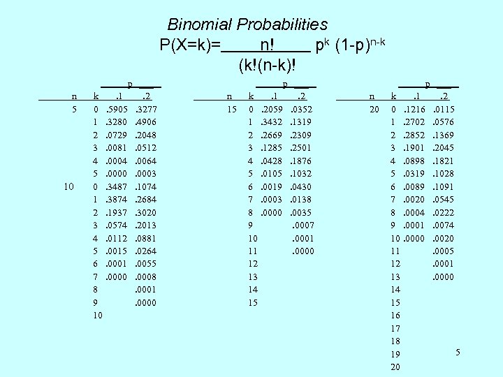
Binomial Probabilities P(X=k)= n! pk (1 -p)n-k (k!(n-k)! n 5 10 k 0 1 2 3 4 5 6 7 8 9 10 p ___. 1. 2. 5905. 3277. 3280. 4906. 0729. 2048. 0081. 0512. 0004. 0064. 0000. 0003. 3487. 1074. 3874. 2684. 1937. 3020. 0574. 2013. 0112. 0881. 0015. 0264. 0001. 0055. 0000. 0008. 0001. 0000 n 15 p ___ k. 1. 2 0. 2059. 0352 1. 3432. 1319 2. 2669. 2309 3. 1285. 2501 4. 0428. 1876 5. 0105. 1032 6. 0019. 0430 7. 0003. 0138 8. 0000. 0035 9. 0007 10. 0001 11. 0000 12 13 14 15 n 20 p ___ k. 1. 2 0. 1216. 0115 1. 2702. 0576 2. 2852. 1369 3. 1901. 2045 4. 0898. 1821 5. 0319. 1028 6. 0089. 1091 7. 0020. 0545 8. 0004. 0222 9. 0001. 0074 10. 0000. 0020 11. 0005 12. 0001 13. 0000 14 15 16 17 18 5 19 20

Example: Estimating % Yellow M&M Choose a partner in the class. I have a population of M & Ms. The percentage of yellow M & Ms is either p=10% or p=20%. You have been hired as a statistical consultant to decide whether the true percentage of yellow M & Ms is 10%. Here is your decision table with associated payoffs/losses. TRUE STATE OF THE BAG H 0 is true: p=10% H 0 is false: p=20% Decision Fail to reject H 0 Your boss gives you a bonus, You lose your job, and you and Dalene buys you lunch. and you must buy Dalene lunch. Reject H 0 You lose your job, and you must buy Dalene lunch. Your boss gives you a bonus, and Dalene buys you lunch. I will show you a random sample from the bag, but you must pay 20 cents for each M & M you see, and you must buy M & Ms in $1 increments. That is, you may see 5, 10, 15, or 20 M & Ms. 6
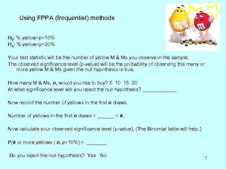
Using FPPA (frequentist) methods H 0: % yellow=p=10% HA: % yellow=p=20% Your test statistic will be the number of yellow M & Ms you observe in the sample. The observed significance level (p-value) will be the probability of observing this many or more yellow M & Ms given the null hypothesis is true. How many M & Ms, n, would you like to buy? 5 10 15 20 At what significance level will you reject the null hypothesis? ______ Now record the number of yellows in the first n draws. Number of yellows in the first n draws = ______ = k. Now calculate your observed significance level (p-value). (The Binomial table will help. ) P(k or more yellows | n, p=10%) = _______ Do you reject the null hypothesis? Yes No 7
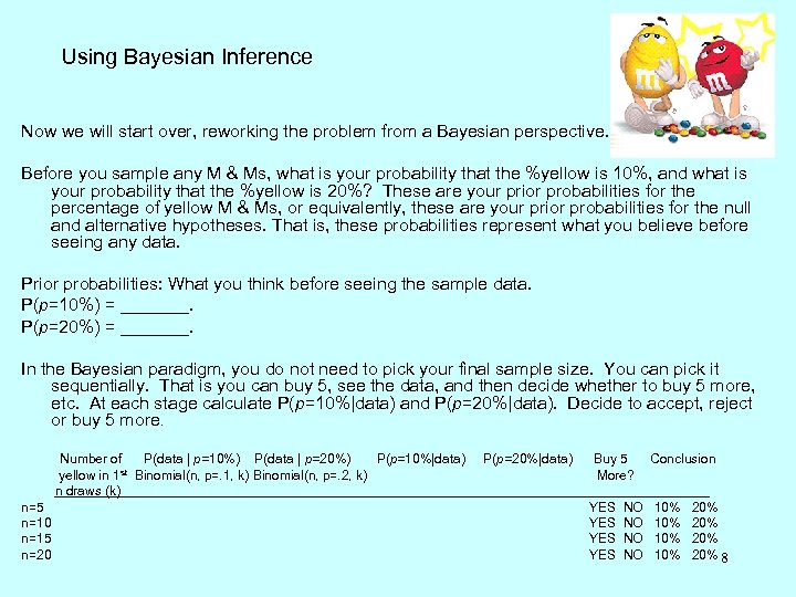
Using Bayesian Inference Now we will start over, reworking the problem from a Bayesian perspective. Before you sample any M & Ms, what is your probability that the %yellow is 10%, and what is your probability that the %yellow is 20%? These are your prior probabilities for the percentage of yellow M & Ms, or equivalently, these are your prior probabilities for the null and alternative hypotheses. That is, these probabilities represent what you believe before seeing any data. Prior probabilities: What you think before seeing the sample data. P(p=10%) = _______. P(p=20%) = _______. In the Bayesian paradigm, you do not need to pick your final sample size. You can pick it sequentially. That is you can buy 5, see the data, and then decide whether to buy 5 more, etc. At each stage calculate P(p=10%|data) and P(p=20%|data). Decide to accept, reject or buy 5 more. Number of P(data | p=10%) P(data | p=20%) P(p=10%|data) P(p=20%|data) Buy 5 Conclusion yellow in 1 st Binomial(n, p=. 1, k) Binomial(n, p=. 2, k) n draws (k) n=5 n=10 n=15 n=20 More? _______ YES NO 10% 20% 8
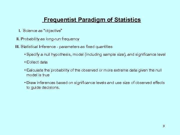
Frequentist Paradigm of Statistics I. Science as “objective” II. Probability as long-run frequency III. Statistical Inference - parameters as fixed quantities • Specify a null hypothesis, model (including sample size), and significance level • Collect data • Calculate the probability of the observed or more extreme data given the null model is true • Draw inferences based on significance levels and use size of observed effects to guide decisions. 9
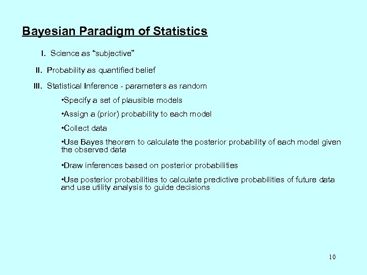
Bayesian Paradigm of Statistics I. Science as “subjective” II. Probability as quantified belief III. Statistical Inference - parameters as random • Specify a set of plausible models • Assign a (prior) probability to each model • Collect data • Use Bayes theorem to calculate the posterior probability of each model given the observed data • Draw inferences based on posterior probabilities • Use posterior probabilities to calculate predictive probabilities of future data and use utility analysis to guide decisions 10
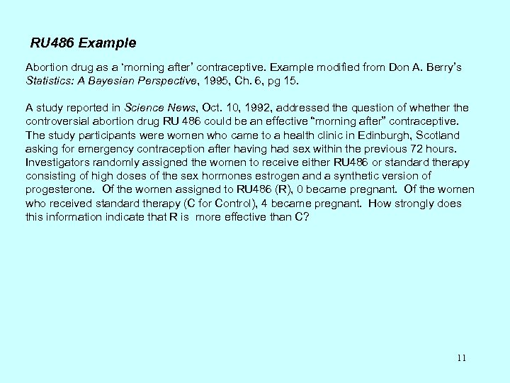
RU 486 Example Abortion drug as a ‘morning after’ contraceptive. Example modified from Don A. Berry’s Statistics: A Bayesian Perspective, 1995, Ch. 6, pg 15. A study reported in Science News, Oct. 10, 1992, addressed the question of whether the controversial abortion drug RU 486 could be an effective “morning after” contraceptive. The study participants were women who came to a health clinic in Edinburgh, Scotland asking for emergency contraception after having had sex within the previous 72 hours. Investigators randomly assigned the women to receive either RU 486 or standard therapy consisting of high doses of the sex hormones estrogen and a synthetic version of progesterone. Of the women assigned to RU 486 (R), 0 became pregnant. Of the women who received standard therapy (C for Control), 4 became pregnant. How strongly does this information indicate that R is more effective than C? 11
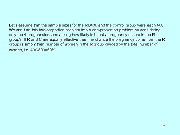
Let’s assume that the sample sizes for the RU 486 and the control group were each 400. We can turn this two-proportion problem into a one-proportion problem by considering only the 4 pregnancies, and asking how likely is it that a pregnancy occurs in the R group? If R and C are equally effective then the chance the pregnancy come from the R group is simply then number of women in the R group divided by the total number of women, i. e. 400/800=50%. 12
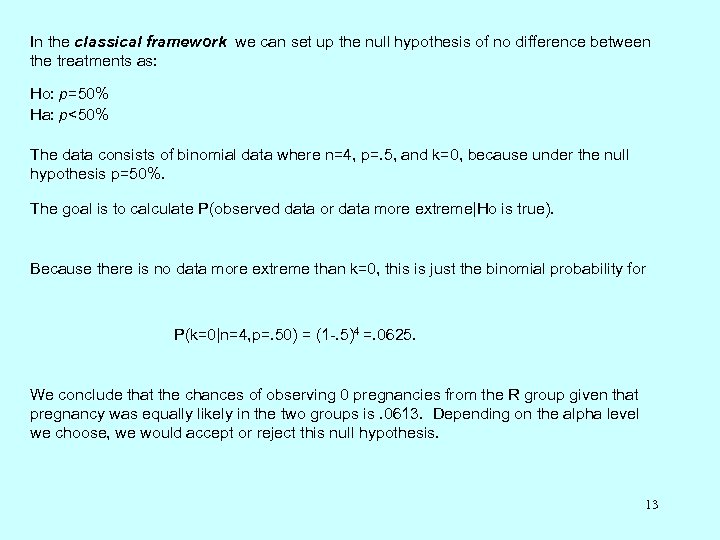
In the classical framework we can set up the null hypothesis of no difference between the treatments as: Ho: p=50% Ha: p<50% The data consists of binomial data where n=4, p=. 5, and k=0, because under the null hypothesis p=50%. The goal is to calculate P(observed data or data more extreme|Ho is true). Because there is no data more extreme than k=0, this is just the binomial probability for P(k=0|n=4, p=. 50) = (1 -. 5)4 =. 0625. We conclude that the chances of observing 0 pregnancies from the R group given that pregnancy was equally likely in the two groups is. 0613. Depending on the alpha level we choose, we would accept or reject this null hypothesis. 13
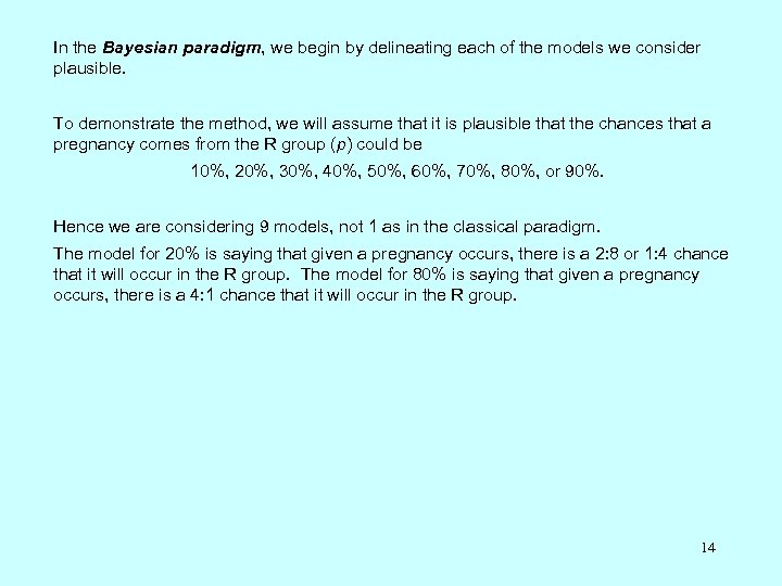
In the Bayesian paradigm, we begin by delineating each of the models we consider plausible. To demonstrate the method, we will assume that it is plausible that the chances that a pregnancy comes from the R group (p) could be 10%, 20%, 30%, 40%, 50%, 60%, 70%, 80%, or 90%. Hence we are considering 9 models, not 1 as in the classical paradigm. The model for 20% is saying that given a pregnancy occurs, there is a 2: 8 or 1: 4 chance that it will occur in the R group. The model for 80% is saying that given a pregnancy occurs, there is a 4: 1 chance that it will occur in the R group. 14
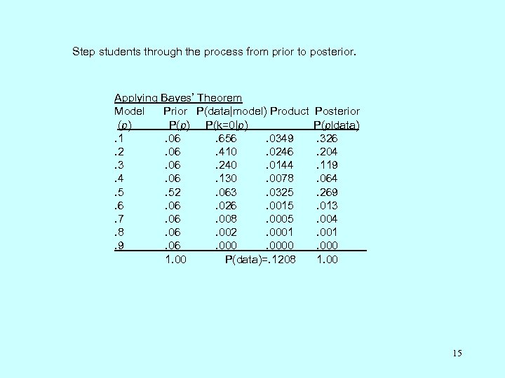
Step students through the process from prior to posterior. Applying Bayes’ Theorem Model Prior P(data|model) Product Posterior (p) P(p) P(k=0|p) P(pldata). 1. 06. 656. 0349. 326. 2. 06. 410. 0246. 204. 3. 06. 240. 0144. 119. 4. 06. 130. 0078. 064. 5. 52. 063. 0325. 269. 6. 026. 0015. 013. 7. 06. 008. 0005. 004. 8. 06. 002. 0001. 9. 06. 0000. 000 1. 00 P(data)=. 1208 1. 00 15
• From column 5 we can make the statement, the posterior probability that p=. 1 is 32. 6%. This model, p=. 1, has the highest posterior probability. • Notice that these posterior probabilities sum to 1, and in calculating them we considered only the data we observed. Data more extreme than that observed data plays no part in the Bayesian paradigm. • Also note, that the probability that p=. 5 dropped from 52% in the prior, to about 27% in the posterior. This demonstrates how we update our beliefs based on observed data. 16
The Bayesian paradigm allows us to make direct probability statements about our models. We can also calculate the probability that RU 486 is more effective than the control treatment. This event corresponds to the sum of the models where p<. 5. By summing the posterior probabilities for these 4 models, we get the probability that RU 486 is more effective is 32. 6%+20. 4%+11. 9%+6. 4%=71. 3%. 17
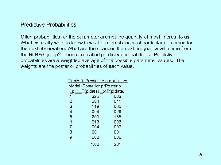
Predictive Probabilities Often probabilities for the parameter are not the quantity of most interest to us. What we really want to know is what are the chances of particular outcomes for the next observation. What are the chances the next pregnancy will come from the RU 486 group? These are called predictive probabilities. Predictive probabilities are a weighted average of the possible parameter values. The weights are the posterior probabilities of each value. Table 5. Predictive probabilities Model Posterior p*Posterior _p___P(pldata) _p*P(p|data). 1. 326. 033. 2. 204. 041. 3. 119. 036. 4. 064. 026. 5. 269. 135. 6. 013. 008. 7. 004. 003. 8. 001. 9. 000 1. 00 . 281 18
In this example we considered only 9 possible values for p. Using calculus, we can consider any value of p between 0 and 1. This simply requires us to use integration rather than summations in the calculations presented above. Next time I’ll show you how to do this in simple models in which you can circumvent the calculus. 19
394d87cc79139373840e6cb7947aaaf9.ppt