3ef91dfc9f4472f70b7022c15e126361.ppt
- Количество слайдов: 137
Bayesian data analysis 1 using Bugs 2 and R 3 1 Fit complicated models 2 easily 3 display . . and understand results. 1
Bayesian data analysis using BUGS and R Prof. Andrew Gelman Dept. of Statistics and Political Science Columbia University Robert Wood Johnson Health and Society Scholars Program February 22 -23, 2006 2

Introduction to the course 3
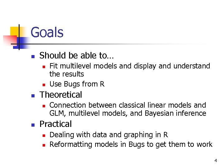
Goals n Should be able to… n n n Theoretical n n Fit multilevel models and display and understand the results Use Bugs from R Connection between classical linear models and GLM, multilevel models, and Bayesian inference Practical n n Dealing with data and graphing in R Reformatting models in Bugs to get them to work 4
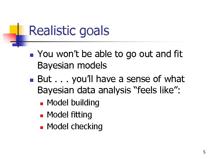
Realistic goals n n You won’t be able to go out and fit Bayesian models But. . . you’ll have a sense of what Bayesian data analysis “feels like”: n n n Model building Model fitting Model checking 5
Overview n n n What is Bayesian data analysis? Why Bayes? Why R and Bugs [schools example] Hierarchical linear regression [radon example] Bayesian data analysis: what it is and what it is not [several examples] Model checking [several examples] Hierarchical Poisson regression [police stops example] Understanding the Gibbs sampler and Metropolis algorithm Computation [social networks example] Troubleshooting: simulations don’t work, run too slowly, make no sense Accounting for data collection [pre-election polling example] If there is time: hierarchical logistic regression with varying intercepts and slopes [red/blue states example] Loose ends 6

Structure of this course n n n Main narrative on powerpoint Formulas on blackboard On my computer and yours: n n n Bugs, R, and a text editor Data, Bugs models, and R scripts for the examples We do computer demos together Pause to work on your own to play with the models—we then discuss together Lecturing for motivating examples Interrupt to ask questions 7
Structure of this course n Several examples. For each: n n n Understanding how Bugs works and how to work with Bugs More examples n n Set up the Bugs model Use R to set up the data and initial values, and to run Bugs Use R to understand the inferences Play with variations on your own computer Working around problems in Bugs Using the inferences to answer real questions Not much theory. If you want more theory, let me know! Emphasis on general methods for model construction, expansion, patching, and understanding 8

Introduction to Bayes 9
What is Bayesian data analysis? Why Bayes? n Effective and flexible n n Modular (“Tinkertoy”) approach Combines information from different sources Estimate inferences without overfitting for models with large number of parameters Examples from sample surveys and public health include: n Small-area estimation, longitudinal data analysis, and multilevel regression 10
What are BUGS and R? n Bugs n n n R n n Fit Bayesian statistical models No programming required Open source language for statistical computing and graphics Bugs from R n n Offers flexibility in data manipulation before the analysis and display of inferences after Avoids tedious issues of working with Bugs directly [Open R: schools example] 11
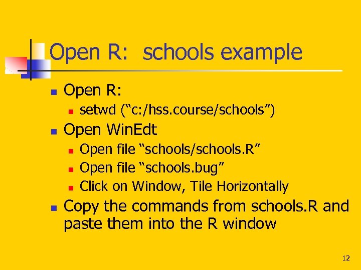
Open R: schools example n Open R: n n Open Win. Edt n n setwd (“c: /hss. course/schools”) Open file “schools/schools. R” Open file “schools. bug” Click on Window, Tile Horizontally Copy the commands from schools. R and paste them into the R window 12
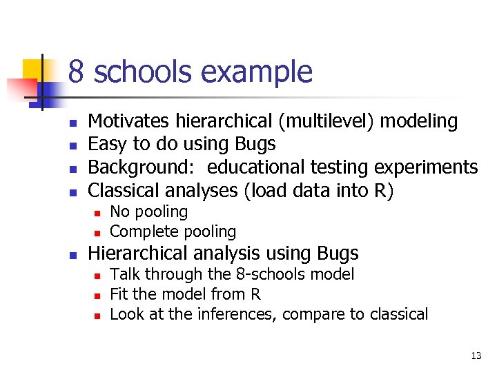
8 schools example n n Motivates hierarchical (multilevel) modeling Easy to do using Bugs Background: educational testing experiments Classical analyses (load data into R) n n n No pooling Complete pooling Hierarchical analysis using Bugs n n n Talk through the 8 -schools model Fit the model from R Look at the inferences, compare to classical 13
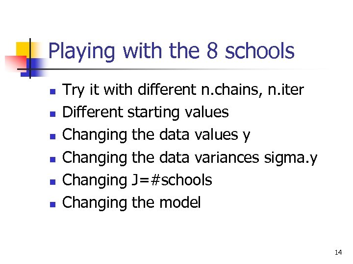
Playing with the 8 schools n n n Try it with different n. chains, n. iter Different starting values Changing the data values y Changing the data variances sigma. y Changing J=#schools Changing the model 14
End 8 -schools example 15
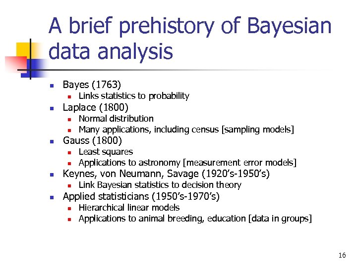
A brief prehistory of Bayesian data analysis n Bayes (1763) n n Laplace (1800) n n Least squares Applications to astronomy [measurement error models] Keynes, von Neumann, Savage (1920’s-1950’s) n n Normal distribution Many applications, including census [sampling models] Gauss (1800) n n Links statistics to probability Link Bayesian statistics to decision theory Applied statisticians (1950’s-1970’s) n n Hierarchical linear models Applications to animal breeding, education [data in groups] 16
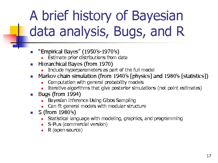
A brief history of Bayesian data analysis, Bugs, and R n “Empirical Bayes” (1950’s-1970’s) n n Hierarchical Bayes (from 1970) n n n Computation with general probability models Iterative algorithms that give posterior simulations (not point estimates) Bugs (from 1994) n n n Include hyperparameters as part of the full model Markov chain simulation (from 1940’s [physics] and 1980’s [statistics]) n n Estimate prior distributions from data Bayesian inference Using Gibbs Sampling Can fit general models with modular structure S (from 1980’s) n n n Statistical language with modeling, graphics, and programming S-Plus (commercial version) R (open-source) 17
My own experiences with Bayes, Bugs, and R n n n Bayesian methods really work, especially for models with lots of parameters Use R for data manipulations and simple models Use Bugs (from R) as first try in fitting complex models Use R to make graphs to check that fitted model makes sense When Bugs doesn’t work, program in R directly 18
Bayesian regression using Bugs 19
R and Bugs for classical inference Radon example n Fitting a linear regression in Bugs n Displaying the results in R n Complete-pooling and no-pooling models n Model extensions [open R: radon example] n 20
Open R: radon example n In Win. Edt n n n Open file “radon/radon_setup. R” We’ll talk through the code In R: n n n setwd (“. . /radon”) source (“radon_setup. R”) Regression output will appear on the R console and graphics windows 21
Fitting a linear regression in R and Bugs n n The Bugs model Setting up data and initial values in R Running Bugs and checking convergence Displaying the fitted line and residuals in R 22
Radon example in R (complete pooling) n In Win. Edt n n n Open file “radon/radon. classical 1. R” In other window, open file “radon. classical. bug” Copy the commands (one paragraph at a time) from radon. classical 1. R and paste them into the R window n n Fit the model Plot the data and estimates Plot the residuals (two versions) Label the plot 23
Simple extensions of the radon model n n n Separate variances for houses with and without basements t instead of normal errors Fitting each model, then understanding it 24
Radon regression with 2 variance parameters n Separate variances for houses with and without basements n n n Bugs model Setting it up in R Using the posterior inferences to compare the two variance parameters 25
Radon example in R (regression with 2 variance parameters) n In Win. Edt n n n Open file “radon/radon. extend. 1. R” Other window, open file “radon. classical. 2 vars. bug” Copy from radon. extend. 1. R and paste into the R window n n Fit the model Display a posterior inference Compute a posterior probability STOP 26
Robust regression for radon data n t instead of normal errors n n n Issues with the degrees-of-freedom parameter Looking at the posterior simulations and comparing to the prior distribution Interpreting the scale parameter 27
Radon example in R (robust regression using the t model) n In Win. Edt n n n Stay with “radon/radon. extend. 1. R” Other window: “radon. classical. t. bug” Copy rest of radon. extend. 1. R and paste into the R window n n n Fit the t model Run again with n. iter=1000 iterations Make some plots 28
Fit your own model to the radon data Alter the Bugs model n Change the setup in R n Run the model and check convergence n Display the posterior inferences in R [Suggestions of alternative models? ] n 29
Fitting several regressions in R and Bugs n Back to the radon example n n n Complete pooling [we just did] No pooling [do now: see next slide] Bugs model is unchanged Fit separate model in each county and save them as a list Displaying data and fitted lines from 11 counties Next step: hierarchical regression 30
Radon example in R (no pooling) n In Win. Edt n n n Open file “radon/radon. classical 2. R” In other window, open file “radon. classical. bug” Copy from radon. classical 2. R and paste into the R window n n Fit the model (looping through n. county=11 counties) Plot the data and estimates Plot the residuals (two versions) Label the plot 31
![Hierarchical linear regression: models [Show the models on blackboard] n Generalizing the Bugs model Hierarchical linear regression: models [Show the models on blackboard] n Generalizing the Bugs model](https://present5.com/presentation/3ef91dfc9f4472f70b7022c15e126361/image-32.jpg)
Hierarchical linear regression: models [Show the models on blackboard] n Generalizing the Bugs model n n n Varying intercepts, varying slopes Adding predictors at the group level Also write each model using algebra More than one way to write (or program) each model 32
![Hierarchical linear regression: fitting and understanding [working on blackboard] n Displaying results in R Hierarchical linear regression: fitting and understanding [working on blackboard] n Displaying results in R](https://present5.com/presentation/3ef91dfc9f4472f70b7022c15e126361/image-33.jpg)
Hierarchical linear regression: fitting and understanding [working on blackboard] n Displaying results in R n Comparing models n n Interpreting coefficients and variance parameters Going beyond R 2 33
Hierarchical linear regression: varying intercepts n n Example: county-level variation for radon Recall classical models n n n Including county effects hierarchically n n Complete pooling No pooling (separate regressions) Bugs model Written version More than one way to write the model Fitting and understanding n n Interpreting the parameters Displaying results in R 34
Radon example in R (varying intercepts) n In Win. Edt n n n “radon/radon. multilevel. 1. R” Other window: “radon. multilevel. 1. bug” Copy from radon. multilevel. 1. R and paste into the R window n n n Fit the model (debug=TRUE) Close the Bugs window Run for 100, then 1000 iterations Plot the data and estimates for 11 counties Plot all 11 regression lines at once 35
Hierarchical linear regression: varying intercepts, varying slopes n The model n n n Bugs model Written version Setup in R Running Bugs, checking convergence Displaying the fitted model in R Understanding the new parameters 36
Radon example in R (varying intercepts and slopes) n In Win. Edt n n n “radon/radon. multilevel. 2. R” Other window: “radon. multilevel. 2. bug” Copy from radon. multilevel. 2. R and paste into the R window n n n Fit the model (debug=TRUE) Close the Bugs window Run for 500 iterations Plot the data and estimates for 11 counties Plot all 11 regression lines at once Plot slopes vs. intercepts 37
Playing with hierarchical modeling for the radon example n n Uranium level as a county-level predictor Changing the sample sizes Perturbing the data Fitting nonlinear models 38
Radon example in R (adding a county-level predictor) n In Win. Edt n n n radon/radon. multilevel. 3. R Other window: radon. multilevel. 3. bug Copy from radon. multilevel. 3. R and paste into the R window n n Fit the model Plot the data and estimates for 11 counties Plot all 11 regression lines at once Plot county parameters vs. county uranium level 39
Varying intercepts and slopes with correlated group-level errors n The model n n n Statistical notation Bugs model Show on blackboard Correlation and group-level predictors More in chapters 13 and 17 of Gelman and Hill (2006) 40
End radon example 41
Bayesian data analysis: what it is and what it is not 42
Bayesian data analysis: it is and what it is not n Popular view of Bayesian statistics n n n Subjective probability Elicited prior distributions Bayesian data analysis as we do it n n n what Hierarchical modeling Many applications Conceptual framework n n n Fit a probability model to data Check fit, ride the model as far as it will take you Improve/expand/extend model 43
Overview of Bayesian data analysis n n n n Decision analysis for home radon Where did the “prior distribution” come from? Quotes illustrating misconceptions of Bayesian inference State-level opinions from national polls (hierarchical modeling and validation) Serial dilution assay (handling uncertainty in a nonlinear model) Simulation-based model checking Some open problems in BDA 44
Decision analysis for home radon n Radon gas n n n Radon webpage n n n Causes 15, 000 lung cancers per year in U. S. Comes from underground; home exposure http: //www. stat. columbia. edu/~radon/ Click for recommended decision Bayesian inference n n Prior + data = posterior Where did the prior distribution come from? 45
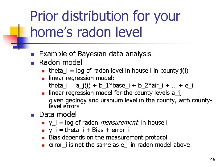
Prior distribution for your home’s radon level n n Example of Bayesian data analysis Radon model n n theta_i = log of radon level in house i in county j(i) linear regression model: theta_i = a_j(i) + b_1*base_i + b_2*air_i + … + e_i linear regression model for the county levels a_j, given geology and uranium level in the county, with countylevel errors Data model n n y_i = log of radon measurement in house i y_i = theta_i + Bias + error_i Bias depends on the measurement protocol error_i is not the same as e_i in radon model above 46
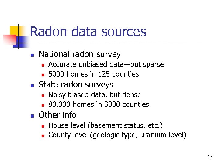
Radon data sources n National radon survey n n n State radon surveys n n n Accurate unbiased data—but sparse 5000 homes in 125 counties Noisy biased data, but dense 80, 000 homes in 3000 counties Other info n n House level (basement status, etc. ) County level (geologic type, uranium level) 47
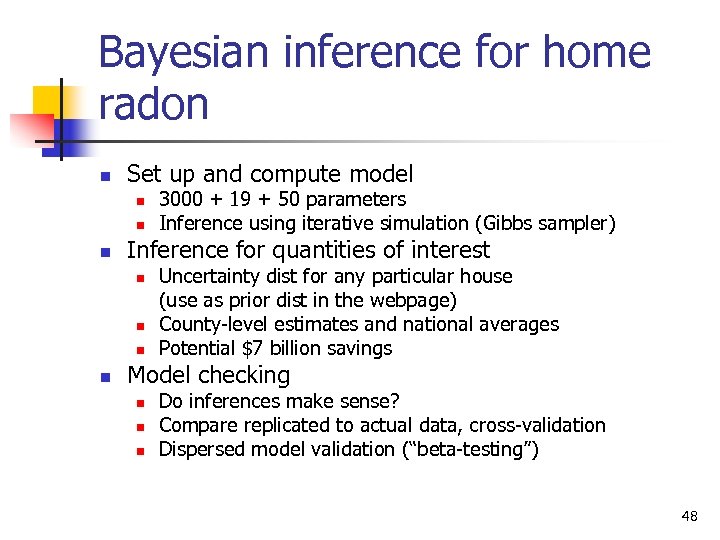
Bayesian inference for home radon n Set up and compute model n n n Inference for quantities of interest n n 3000 + 19 + 50 parameters Inference using iterative simulation (Gibbs sampler) Uncertainty dist for any particular house (use as prior dist in the webpage) County-level estimates and national averages Potential $7 billion savings Model checking n n n Do inferences make sense? Compare replicated to actual data, cross-validation Dispersed model validation (“beta-testing”) 48
Bayesian inference for home radon n n Allows estimation of over 3000 parameters Summarizes uncertainties using probability Combines data sources Model is testable (falsifiable) 49

End radon example 50
Pro-Bayesian quotes n n Hox (2002): “In classical statistics, the population parameter has only one specific value, only we happen not to know it. In Bayesian statistics, we consider a probability distribution of possible values for the unknown population distribution. ” Somebody’s webpage: “To a true subjective Bayesian statistician, the prior distribution represents the degree of belief that the statistician or client has in the value of the unknown parameter. . . it is the responsibility of the statistician to elicit the true beliefs of the client. ” 51
Why these views of Bayesian statistics are wrong! n Hox quote (distribution of parameter values) n n n Our response: parameter values are “fixed but unknown” in Bayesian inference also! Confusion between quantities of interest and inferential summaries Anonymous quote n n Our response: the statistical model is an assumption to be held if useful Confusion between statistical analysis and decision making 52
Anti-Bayesian quotes n n Efron (1986): “Bayesian theory requires a great deal of thought about the given situation to apply sensibly. ” Ehrenberg (1986): “Bayesianism assumes: (a) Either a weak or uniform prior, in which case why bother? , (b) Or a strong prior, in which case why collect new data? , (c) Or more realistically, something in between, in which case Bayesianism always seems to duck the issue. ” 53
Why these views of Bayesian statistics are wrong! n Efron quote (difficulty of Bayes) n n n Our response: demonstration that Bayes solves many problems more easily that other methods Mistaken focus on the simplest problems Ehrenberg quote (arbitrariness of prior dist) n n Our response: the “prior dist” represents the information provided by a group-level analysis One “prior dist” serves many analyses 54
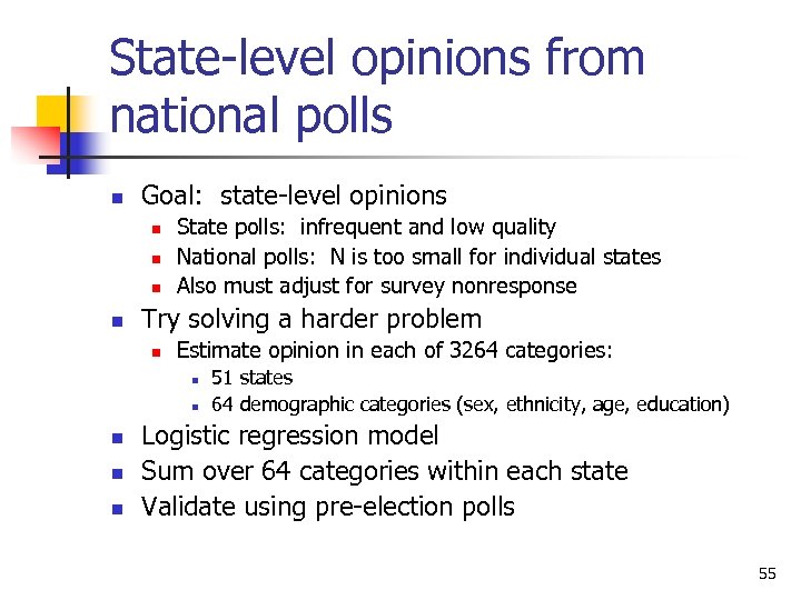
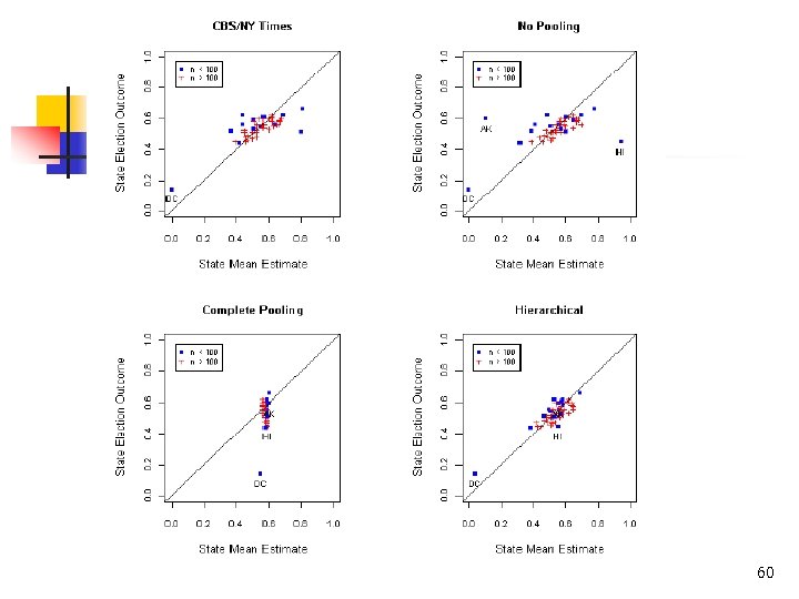
State-level opinions from national polls n Goal: state-level opinions n n State polls: infrequent and low quality National polls: N is too small for individual states Also must adjust for survey nonresponse Try solving a harder problem n Estimate opinion in each of 3264 categories: n n n 51 states 64 demographic categories (sex, ethnicity, age, education) Logistic regression model Sum over 64 categories within each state Validate using pre-election polls 55
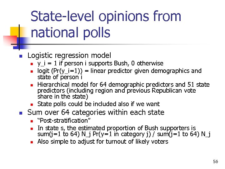
State-level opinions from national polls n Logistic regression model n n n y_i = 1 if person i supports Bush, 0 otherwise logit (Pr(y_i=1)) = linear predictor given demographics and state of person i Hierarchical model for 64 demographic predictors and 51 state predictors (including region and previous Republican vote share in the state) State polls could be included also if we want Sum over 64 categories within each state n n n “Post-stratification” In state s, the estimated proportion of Bush supporters is sum(j=1 to 64) N_j Pr(y=1 in category j) / sum(j=1 to 64) N_j Also simple to adjust for turnout of likely voters 56
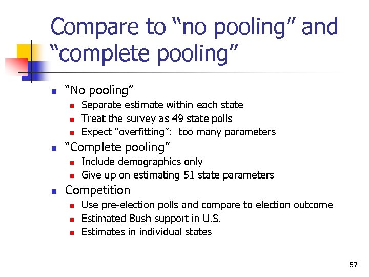
Compare to “no pooling” and “complete pooling” n “No pooling” n n “Complete pooling” n n n Separate estimate within each state Treat the survey as 49 state polls Expect “overfitting”: too many parameters Include demographics only Give up on estimating 51 state parameters Competition n Use pre-election polls and compare to election outcome Estimated Bush support in U. S. Estimates in individual states 57
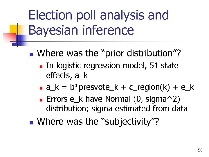
Election poll analysis and Bayesian inference n Where was the “prior distribution”? n n In logistic regression model, 51 state effects, a_k = b*presvote_k + c_region(k) + e_k Errors e_k have Normal (0, sigma^2) distribution; sigma estimated from data Where was the “subjectivity”? 58
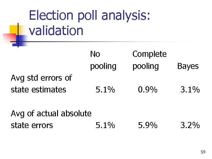
Election poll analysis: validation No pooling Complete pooling Bayes 5. 1% 0. 9% 3. 1% Avg of actual absolute state errors 5. 1% 5. 9% 3. 2% Avg std errors of state estimates 59
60
End pre-election polling example 61
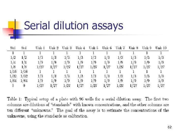
Serial dilution assays 62
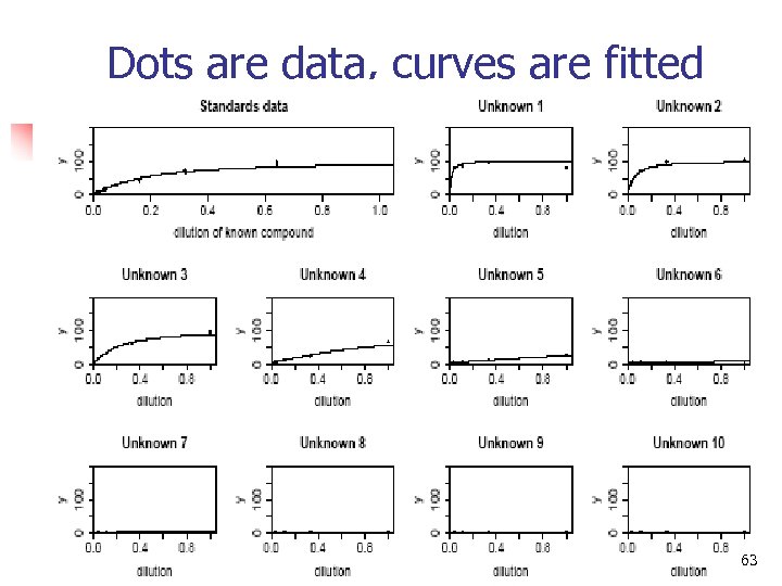
Dots are data, curves are fitted 63
Serial dilution assays: motivation for Bayesian inference n n Classical approach: read the estimate off the calibration curve Difficulties n n n “above detection limit”: curve is too flat “below detection limit”: signal/noise ratio is too low For some samples, all the data are above or below detection limits! Goal: downweight—but don’t discard—weak data Maximum likelihood (weighted least squares) Bayes handles uncertainty in the parameters of the calibration curve 64
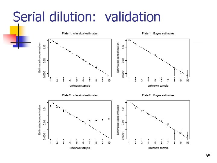
Serial dilution: validation 65

End assays example 66
Summary n n n Bayesian data analysis is about modeling Not an optimization problem; no “loss function” Make a (necessarily) false set of assumptions, then work them hard Complex models --> complex inferences --> lots of places to check model fit Prior distributions are usually not “subjective” and do not represent “belief” Models are applied repeatedly (“beta-testing”) 67

Model checking 68
Model checking n Basic idea: n n n Generalization of classical methods: n n n Display observed data (always a good idea anyway) Simulate several replicated datasets from the estimated model Display the replicated datasets and compare to the observed data Comparison can be graphical or numerical Hypothesis testing Exploratory data analysis Crucial “safety valve” in Bayesian data analysis 69
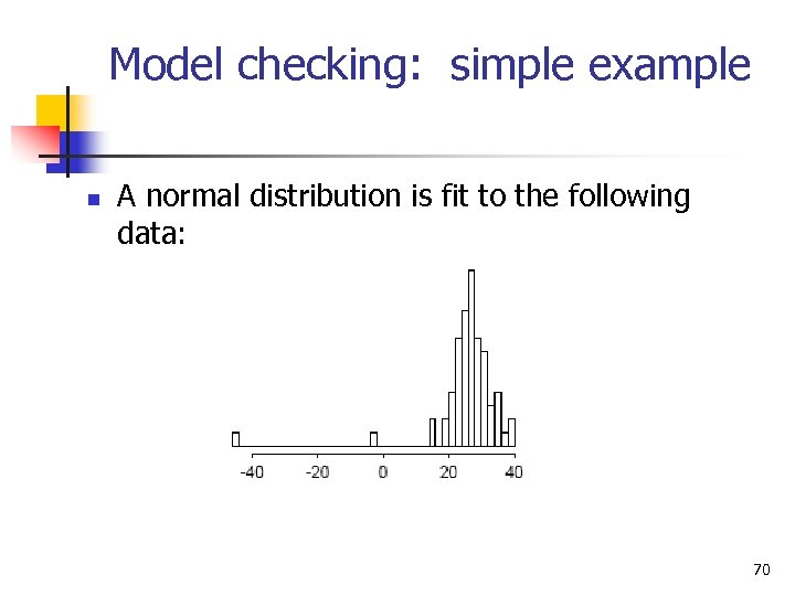
Model checking: simple example n A normal distribution is fit to the following data: 70
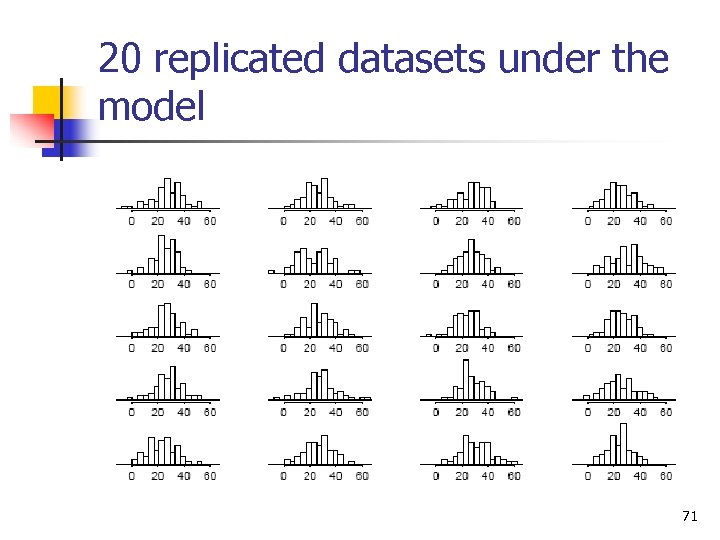
20 replicated datasets under the model 71
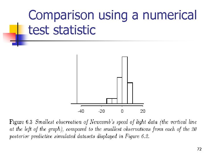
Comparison using a numerical test statistic 72
Model checking: another example n n Logistic regression model fit to data from psychology: a 15 x 23 array of responses for each of 6 persons Next slide shows observed data (at left) and 7 replicated datasets (at right) 73
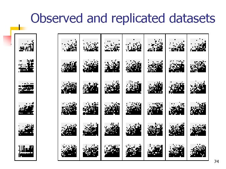
Observed and replicated datasets 74
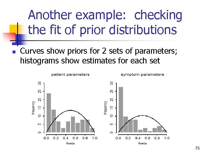
Another example: checking the fit of prior distributions n Curves show priors for 2 sets of parameters; histograms show estimates for each set 75
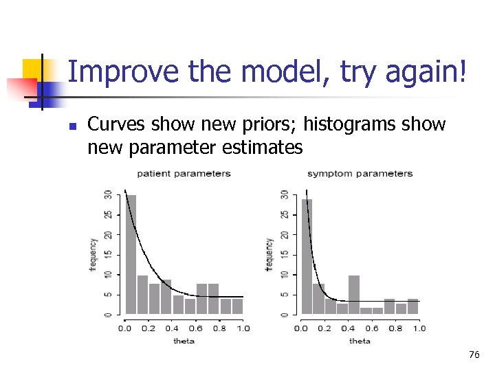
Improve the model, try again! n Curves show new priors; histograms show new parameter estimates 76
Model checking and model comparison n Generalizing classical methods n n n n t tests chi-squared tests F-tests R 2, deviance, AIC Use estimation rather than testing where possible Posterior predictive checks of model fit DIC for predictive model comparison 77
Model checking: posterior predictive tests n n Test statistic T(y) Replicated datasets y. repk, k=1, …, n. sim Compare T(y) to the posterior predictive distribution of T(y. repk) Discrepancy measure T(y, thetak) n n Look at n. sim values of the difference, T(y, thetak) - T(y. repk, thetak) Compare this distribution to 0 78
Model comparison: DIC n n Generalization of “deviance” in classical GLM p_D is effective number of parameters n n n 8 -schools example Radon example DIC is estimated error of out-of-sample predictions DIC = posterior mean of deviance + p_D Radon example 79

More on multilevel modeling 80
Including linear predictors in a hierarchical model n Radon example n n Airflow as a data-level predictor Avg airflow as a county-level predictor Uranium as a county-level predictor How can we include group indicators and a group-level predictor? Example from Advanced Placement study [blackboard] n 81
Hierarchical generalized linear models n Poisson n n Overdispersed n n Example: Police stops Logistic n n n Example: Police stops Example: pre-election polls Other details in this example Other issues n Multinomial logit, robust model 82
Police stop/frisks: example of Poisson regression n n Background on NYPD stops and frisks Data on stops for violent crimes n n n #stops, population, #previous arrests Blacks (African-Americans), Hispanics (Latinos), Whites (European-Americans) Confidentiality: you’re getting fake data In R, compute averages for each group n Variation among precincts? n Poisson regression (count data) [open R: frisk example] n 83
Open R: frisk example n In R: n n In Win. Edt n n n setwd (“. . /frisk”) Open file “frisk/frisk. 0. R” Other window: “frisk. 0. bug” Copy from frisk. 0. R and paste into the R window n n n Read in and look at the data Work with a subset of the data Pre-process Fit the classical Poisson regression in Bugs Fit using “glm” in R, check that results are approx the same 84
Hierarchical Poisson regression for police stops n Poisson regression n n Set up model in Bugs n n Previous arrests as offset Logarithmic link Include precinct predictors Shift batches of parameters to sum to zero Compute the model Slow convergence Compare to aggregate results 85
Frisk example in R (multilevel Poisson regression) n In Win. Edt n n Open file “frisk/frisk. 1. R” Other window: “frisk. 1. bug” Discuss the parts of the model Copy from frisk. 1. R and paste into the R window n n Fit the model Compare to classical Poisson regression 86
Shifting of multilevel regression coefficients n Frisk example: n n n 3 ethnicity coefficients 75 precinct coefficients Subtract mean of each batch n n n See Bugs model “frisk 1. dat” Define new variables g. eth, g. precinct Add the means back to g. 0 87
Overdispersed hierarchical Poisson regression n Use simulations from previous model to test for overdispersion n n n n Chi-squared discrepancy measure Posterior predictive check in R compare observed discrepancy to simulations from replicated data Poisson regression with offset and log link Set up model in Bugs Faster convergence! Display the results in R Compare to non-overdispersed model 88
Frisk example in R (overdispersed model) n In Win. Edt n n Open file “frisk/frisk. 2. R” Other window: “frisk. 2. bug” New variance component for overdispersion Copy from frisk. 2. R and paste into the R window n n Fit the model Compare to non-overdispersed model: n n Coefficient estimates Overdispersion parameter sigma. y 89
Playing with the frisk example n n n Using %black as a precinct-level predictor Looking at other crime types Including previous arrests as a predictor rather than as an offset 90
2 -stage regression for the frisk example n n n #previous arrests is a noisy measure of crime Model 1 of stops given “crime rate” Model 2 of arrests given “crime rate” Each of the 2 models is multilevel, overdisp. “Crime rate” is implicitly estimated by the 2 models simultaneously Set up Bugs model, fit in R 91
Frisk example in R -stage model) n In Win. Edt n n (2 Open file “frisk/frisk. 3. R” Other window: “frisk. 3. bug” Entire model is duplicated: once for stops, once for DCJS arrests Copy from frisk. 3. R and paste into the R window n n Fit the model Compare to previous models 92
End frisk example 93

Computation 94
Understanding the computational method used by Bugs n Key advantages n n n Connections to earlier methods n n n Gives posterior simulations, not a point estimate Works with (almost) any model Maximum likelihood Normal approximation for std errors Multiple imputation Gibbs sampler Metropolis algorithm Difficulties 95
Understanding computation: relation to earlier methods n Maximum likelihood n n +/- std errors n n Hill-climbing algorithm Normal approximation Multiple imputation n Consider parameters as “missing data” [More on blackboard] 96
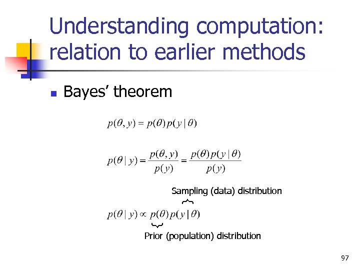
Understanding computation: relation to earlier methods Bayes’ theorem Sampling (data) distribution } Prior (population) distribution 97
Understanding the Gibbs sampler and Metropolis algorithm n Examples of Bugs chains: n Run mcmc. display. R Interpretation as random walks (generalizing maximum likelihood) n Interpretation as iterative imputations (generalizing multiple imputation) [open R: mcmc displays] n 98
Open R: mcmc displays n Open R: n n Open Win. Edt n n setwd (“. . /schools”) Open file “schools/mcmc. display. R” Copy from mcmc. display. R and paste into the R window n n n Read in the function sim. display() Apply it to the schools example In a few minutes, apply it to a previous run of the radon model 99
Understanding the Gibbs sampler and Metropolis algorithm n n n Gibbs sampler as iterative imputations Demonstration on the blackboard for the 8 -schools example Can program directly in R [Appendix C of Bayesian Data Analysis, 2 nd edition] Radon example (graph in R) Conditional updating and the modular structure of Bugs models 100
Understanding the Gibbs sampler and Metropolis algorithm n n n Monitoring convergence Pictures of good and bad convergence [blackboard] n. chains must be at least 2 Role of starting points R-hat n n Less than 1. 1 is good Effective sample size n At least 100 is good 101
Understanding the Gibbs sampler and Metropolis algorithm n n More efficient Gibbs samplers More efficient Metropolis jumping 102
![Special lecture on computation [social networks example] 103 Special lecture on computation [social networks example] 103](https://present5.com/presentation/3ef91dfc9f4472f70b7022c15e126361/image-103.jpg)
Special lecture on computation [social networks example] 103

Troubleshooting 104
Troubleshooting n n n Problems in Bugs Simple Bugs and R solutions Reparameterizing Changing the model slightly Stripping the model down and rebuilding it Expanding the model 105
Troubleshooting: problems and quick solutions n n Problem: model does not compile Solutions: n n n bugs (…, debug=TRUE) Look at where cursor stops in Bugs model Typical problems: n n Go into Bugs user manual n n n Typo, syntax error, illegal use of a distribution or function In Bugs, click on Help, then User manual Check Model Specification and Distributions Go into Bugs examples n n In Bugs, click on Help, then Examples Vol I and II Find an example similar to your problem 106
Troubleshooting: problems and quick solutions n n Problem: model does not run Solutions: n n n bugs (…, debug=TRUE) Look at where cursor stops in Bugs Typical problems: n n Variable in data/inits/params but not in model Variable in model but not in data or params Error in subscripting May need to fix in Bugs model or R script 107
Troubleshooting: problems and quick solutions n n Problem: Trapping in Bugs Solutions: n n Give reasonable starting values for all parameters in the model Make prior distributions more restrictive n n e. g. , dnorm(0, . 01) instead of dnorm(0, . 0001) Change the model slightly n We will discuss some examples 108
Troubleshooting: slow convergence n n Problem: R-hat is still more than 1. 1 for some parameters Solutions: n n n Look at the separate sequences to see what is moving slowly Run Bugs a little longer, possibly using last. value as initial values Reparameterize Change the model slightly Run model on a subset of the data (it’ll go faster) 109
Troubleshooting: reparameterizing n n Nesting predictors Adding redundant additive parameters Adding redundant multiplicative parameters Rescaling n n Example: item response models (hierarchical logistic regressions) for test scores or court votes There is no unique way to write a model 110
Troubleshooting: changing the model slightly n n Normal/t, logit/probit, etc. Bounds on predictions n n n Logistic regression example Use of robust models Approximations to functions n Golf putting [open R: logistic regression example] 111
Open R: logistic regression example n Open R: n n Open Win. Edt n n n setwd (“. . /logit”) Open file “logit/logit. R” Other window: “logit. bug” Copy from logit. R and paste into the R window n n Simulate fake dataset and display it Fit the logistic regression model in R, then Bugs Compare the classical and Bayes estimates Superimpose fitted models on data 112
Logistic regression in R and Bugs: latent-variable parameterization n In Win. Edt n n n Continue looking at “logit. R” Other window: “logit. latent. bug” Copy from logit. R and paste into R n n n Fit logistic regression in Bugs using the latentvariable parameterization Compare the Bugs models, “logit. bug” and “logit. latent. bug” Create an “outlier” in the data and fit logistic regression again 113
Robust logistic regression in Bugs using the t distribution n In Win. Edt n n n Continue looking at “logit. R” Other window: “logit. t. bug”, then “logit. t. df. adj. bug” Copy from logit. R and paste into R n n n Fit latent-variable model with t 4 distribution instead of logistic Fit latent-variable model with tdf distribution (df estimated from data) Fix model to adjust for variance of t distribution 114
Troubleshooting: stripping the model down and rebuilding it n n n Remove interactions, predictors, hierarchical structures Set hyperparameters to fixed values Assign strong prior distributions to hyperparameters 115
Troubleshooting: expanding the model n n Computational problems often indicate statistical problems Adding a variance component n n Adding a hierarchical structure n n Recall Poisson model for frisk data before and after we put in overdispersion Example from analysis of serial dilution data Adding a predictor n Example: including previous election results in an analysis of state-level public opinion 116

Relevance of data collection to statistical analysis 117
Accounting for design of surveys and experiments n General principle n n Include all design info in the analysis Poststratification State-level opinions from national polls Other topics n n n Experiments Cluster sampling Censored data 118
State-level opinions from national polls n Background on pre-election polls n n n Political science Survey methods Survey weighting Classical analysis of a pre-election poll from 1988 n Hierarchical models [Open R: election 88 example] n 119
Open R: election 88 example n Open Win. Edt n n Open file “election 88/election 88_setup. R” In R: n n n setwd (“. . /election 88”) source (“election 88_setup. R”) Data are being loaded in and cleaned 120
Pre-election polls: demographic models n Demographic models n n n n Politically interesting Adjust for nonresponse bias Bugs model Run from R, check convergence Get predictions and sum over states Compare to classical estimates Play with the model yourself 121
Election 88 example in R (demographics only) n Open Win. Edt n n n Open file “election 88/demographics. R” Other window: “demographics. 1. bug”, then “demographics. 2. bug” Copy from demographics. R and paste into R window n n n n Set up and run Bugs model with debug=TRUE Close Bugs window Run Bugs for 100 iterations Run Bugs using model 2 Compute predicted values for each survey respondent Use survey weights to get a weighted avg for each state Compare to raw data and election outcomes 122
Pre-election polls: state models n Hierarchical regressions for states n n n Model with states within regions n n Like the 8 -schools model but with binomial data model Bugs model Run from R, check convergence Get predictions and sum over states Fit nested model, summarize results Compare all the models fit so far 123
Election 88 example in R (states only) n Open Win. Edt n n n Open file “election 88/states. R” Other window: “states. bug” Copy from states. R and paste into R window n n n Set up and run Bugs model Compute estimate for each state Compare to raw data, demographic estimates, and election outcomes 124
Pre-election polls: models with demographics and states n n n Crossed multilevel model with demographic and state coefficients Set up model in Bugs Alternative parameterizations Compare all the models fit so far We’ve used the computational strategy of “subsetting” or “data sampling” 125
Election 88 example in R (demographics and states) n Open Win. Edt n n n Open file “election 88/all. 1. R” Other window: “all. 1. bug” Copy from all. 1. R and paste into the R window n n Set up and run Bugs model Read in Census data (demographics x state) Compute estimate for each state Compare to raw data, demographic estimates, state estimates, and election outcomes 126
Playing with the pre-election polls n n n Including presvote as a state-level predictor Putting Maryland in the northeast Other model alterations? 127
End pre-election polls example 128
Other design and data collection topics n Cluster sampling n n Experiments and observational studies n n n Similar to poststratification, but some clusters are empty (as with Alaska and Hawaii in the preelection polls) Model should be conditional on all design factors Blocking can be treated like clustering Censored data n Include in the likelihood (see chapter 18 of Gelman and Hill, 2006) 129
![Varying-intercept, varyingslope logistic regression n Red/blue states example [if there is time] 130 Varying-intercept, varyingslope logistic regression n Red/blue states example [if there is time] 130](https://present5.com/presentation/3ef91dfc9f4472f70b7022c15e126361/image-130.jpg)
Varying-intercept, varyingslope logistic regression n Red/blue states example [if there is time] 130

Commencement 131
Loose ends n n n n Slow convergence More complicated models Multivariate models, including imputation Huge datasets Suggested improvements in Bugs Indirect nature of Bugs modeling Programming in R [see Appendix C from “Bayesian Data Analysis, ” 2 nd edition] 132
Some open problems in Bayesian data analysis n Complex, highly structured models n n n Computation n (polling example) interactions between states and demographic predictors, modeling changes over time Need reasonable classes of hierarchical models (with “just enough” structure) Algorithms walk through high-dimensional parameter space Key idea: link to computations of simpler models (“multiscale computation”, “simulated tempering”) Model checking n n Automatic graphical displays Estimation of out-of-sample predictive error 133
Concluding discussion n What should you be able to do? n n Set up hierarchical models in Bugs Fit them and display/understand the results using R Use Bugs flexibly to explore models What questions do you have? 134
Software resources n Bugs n n R n n n ? command for quick help from the console Html help (in Help menu) has search function Complete manuals (in Help menu) Webpage (http: //www. r-project. org) has pointers to more help Bugs. R n n User manual (in Help menu) Examples volume 1 and 2 (in Help menu) Webpage (http: //www. mrc-bsu. cam. ac. uk/bugs) has pointers to many more examples and applications Often updated; latest version is always at http: //www. stat. columbia. edu/~gelman/bugs. R/ Appendix C from “Bayesian Data Analysis, ” 2 nd edition, has more examples of Bugs and R programming for the 8 -schools example 135
References General books on Bayesian data analysis Bayesian Data Analysis, 2 nd ed. by A. Gelman, J. Carlin, H. Stern, D. Rubin. CRC Press, 2003. Bayes and Empirical Bayes Methods for Data Analysis by B. Carlin and T. Louis. CRC, 2000. Bayesian Methods: A Social and Behavioral Sciences Approach by Jeff Gill. CRC, 2002. General books on multilevel modeling Hierarchical Linear Models by A. S. Bryk and S. W. Raudenbush. Sage Publications, 2001. Introducing Multilevel Modeling by Ita G G Kreft and Jan de Leeuw. Sage Publications, 1998. Multilevel Analysis by Tom A. B. Snijders and Roel J. Bosker. Sage Publications, 1999. Books on R An R and S Plus Companion to Applied Regression by John Fox. Sage Publications, 2002. Modern Applied Statistics with S by B. Ripley and W. Venables. Springer, 2002. An Introduction to R by W. Venables and D. Smith. Network Theory Ltd, 2002. Books using Bugs Bayesian Statistical Modelling and Applied Bayesian Modelling by P. Congdon. 2001, 2003. References to various specific methods and applications in Gelman et al. (2003). 136
Special thanks The examples were done in collaboration with Donald Rubin, Phillip Price, Jeffrey Fagan, Alex Kiss, Thomas Little, David Park, Joseph Bafumi, Howard Wainer, Zaiying Huang, Ginger Chew, Matt Salganik, and Tian Zheng 137
3ef91dfc9f4472f70b7022c15e126361.ppt