9b309a791ebb7bbaa36db80d8ed61a27.ppt
- Количество слайдов: 14
Basics of Statistical Analysis
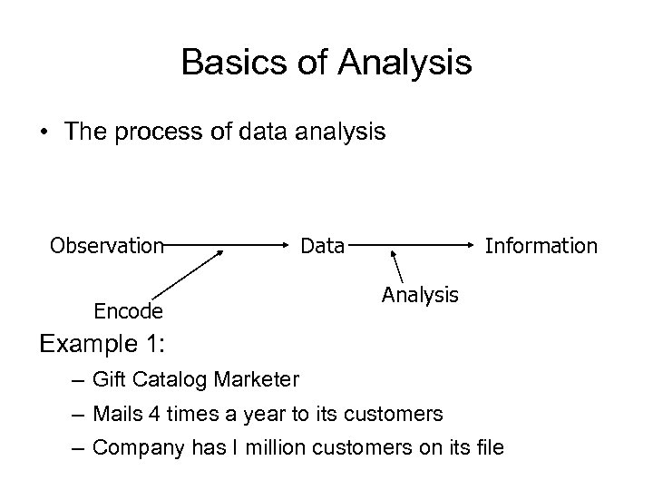
Basics of Analysis • The process of data analysis Observation Encode Data Information Analysis Example 1: – Gift Catalog Marketer – Mails 4 times a year to its customers – Company has I million customers on its file
Example 1 • Cataloger would like to know if new customers buy more than old customers? • Classify New Customers as anyone who brought within the last twelve months. • Analyst takes a sample of 100, 000 customers and notices the following.
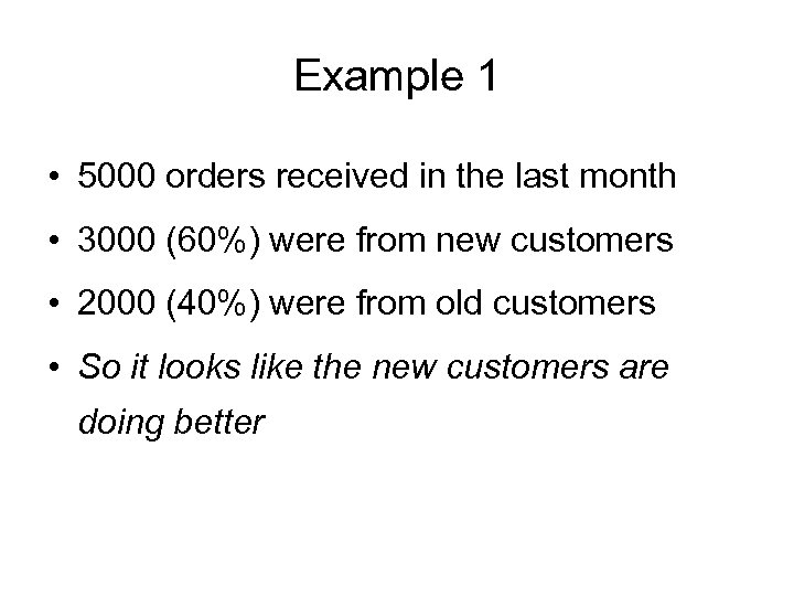
Example 1 • 5000 orders received in the last month • 3000 (60%) were from new customers • 2000 (40%) were from old customers • So it looks like the new customers are doing better
Example 1 • Is there any Catch here!!!!! • Data at this gross level, has no discrimination between customers within either group. – A customer who bought within the last 11 days is treated exactly similar to a customer who bought within the last 11 months.
Example 1 • Can we use some other variable to distinguish between old and new Customers? • Answer: Actual Dollars spent ! • What can we do with this variable? – Find its Mean and Variation. • We might find that the average purchase amount for old customers is two or three times larger than the average among new customers
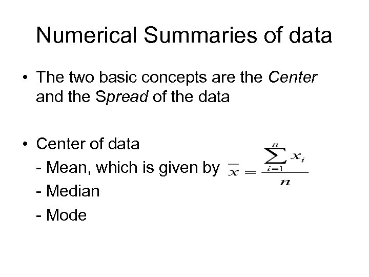
Numerical Summaries of data • The two basic concepts are the Center and the Spread of the data • Center of data - Mean, which is given by - Median - Mode
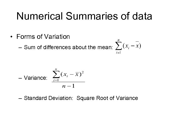
Numerical Summaries of data • Forms of Variation – Sum of differences about the mean: – Variance: – Standard Deviation: Square Root of Variance
Confidence Intervals • In catalog eg, analyst wants to know average purchase amount of customers • He draws two samples of 75 customers each and finds the means to be $68 and $122 • Since difference is large, he draws another 38 samples of 75 each • The mean of means of the 40 samples turns out to be $ 94. 85 • How confident should he be of this mean of means?
Confidence Intervals • Analyst calculates the standard deviation of sample means, called Standard Error (SE) • Basic Premise for confidence Intervals – 95 percent of the time the true mean purchase amount lies between plus or minus 1. 96 standard errors from the mean of the sample means. • C. I. = Mean (+or-) (1. 96) * Standard Error
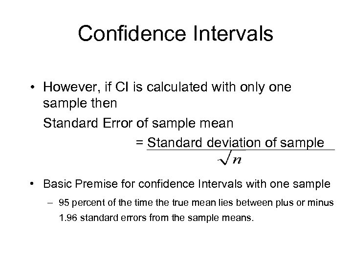
Confidence Intervals • However, if CI is calculated with only one sample then Standard Error of sample mean = Standard deviation of sample • Basic Premise for confidence Intervals with one sample – 95 percent of the time the true mean lies between plus or minus 1. 96 standard errors from the sample means.
Example 2: Confidence Intervals for response rates • You are the marketing analyst for Online Apparel Company • You want to run a promotion for all customers on your database • In the past you have run many such promotions • Historically you needed a 4. 5% response for the promotions to break-even • You want to test the viability of the current fullscale promotion by running a small test promotion
Example 2: Confidence Intervals for response rates • Test 1, 000 names selected at random from the full list. • You construct CI based on required rate of 4. 5% and n=1000 • Confidence Interval= Expected Response ± 1. 96*SE • The SE=. 00655, and CI is (. 0322, . 0578) • In our case C. I. = 3. 22 % to 5. 78%. Thus any response between 3. 22 and 5. 78 % supports hypothesis that true response rate is 4. 5% © 2007 Prentice Hall 16 -13
Example 2: Confidence Intervals for response rates • The list is mailed and actually pulls in 3. 5% • Thus, the true response rate maybe 4. 5% • What if the actual rate pulled in were 5% ? • Regression towards mean: Phenomenon of test result being different from true result • Give more thought to lists whose cutoff rates lie within confidence interval
9b309a791ebb7bbaa36db80d8ed61a27.ppt