Basic Microeconomic Tools Chapter 2 Basic Microeconomic Tools

Basic Microeconomic Tools Chapter 2: Basic Microeconomic Tools 1

Efficiency and Market Performance • Contrast two polar cases – perfect competition – monopoly • What is efficiency? – no reallocation of the available resources makes one economic agent better off without making some other economic agent worse off – example: given an initial distribution of food aid will trade between recipients improve efficiency? Chapter 2: Basic Microeconomic Tools 2

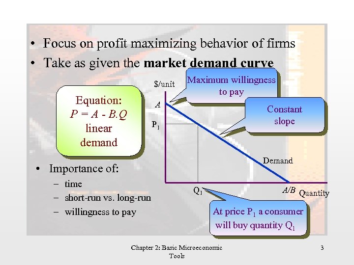
• Focus on profit maximizing behavior of firms • Take as given the market demand curve $/unit Equation: P = A - B. Q linear demand Maximum willingness to pay A Constant slope P 1 Demand • Importance of: – time – short-run vs. long-run – willingness to pay Q 1 A/B Quantity At price P 1 a consumer will buy quantity Q 1 Chapter 2: Basic Microeconomic Tools 3

Perfect Competition • Firms and consumers are price-takers • Firm can sell as much as it likes at the ruling market price – do not need many firms – do need the idea that firms believe that their actions will not affect the market price • Therefore, marginal revenue equals price • To maximize profit a firm of any type must equate marginal revenue with marginal cost • So in perfect competition price equals marginal cost Chapter 2: Basic Microeconomic Tools 4

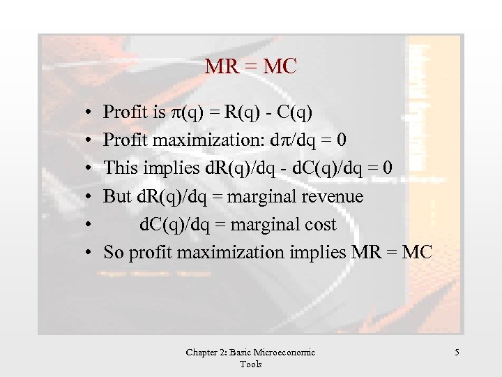
MR = MC • • • Profit is p(q) = R(q) - C(q) Profit maximization: dp/dq = 0 This implies d. R(q)/dq - d. C(q)/dq = 0 But d. R(q)/dq = marginal revenue d. C(q)/dq = marginal cost So profit maximization implies MR = MC Chapter 2: Basic Microeconomic Tools 5

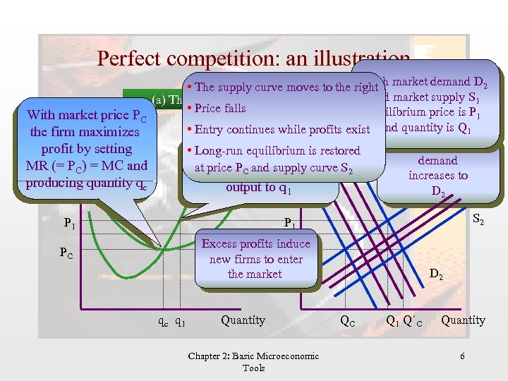
Perfect competition: an illustration With market price PC $/unit the firm maximizes profit by setting MR (= PC) = MC and producing quantity qc With • The supply curve moves to the right market demand D 2 With Industry supply S 1 and market (a) The Firm (b) Themarket demand D 1 • Price falls and market supply is 1 P 1 equilibrium price S equilibrium price is PC $/unit • Entry continues while profits exist and quantity is Q 1 and quantity is QCthat Now assume • MC Long-run equilibrium is restored Existing firms maximize demand at price Pby increasing profits C and supply curve S 2 S 1 increases to D 1 output to q 1 AC D 2 P 1 S 2 P 1 Excess profits induce PC new firms to enter the market PC qc q 1 Quantity Chapter 2: Basic Microeconomic Tools D 2 QC Q 1 Q´C Quantity 6

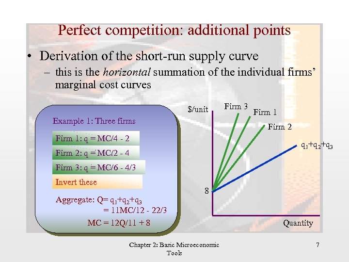
Perfect competition: additional points • Derivation of the short-run supply curve – this is the horizontal summation of the individual firms’ marginal cost curves $/unit Example 1: Three firms Firm 3 Firm 1 Firm 2 Firm 1: MCMC/4+ 8 q = = 4 q - 2 q 1+q 2+q 3 Firm 2: MCMC/2+ 8 q = = 2 q - 4 Firm 3: MCMC/6+ 8 q = = 6 q - 4/3 Invert these Aggregate: Q= q 1+q 2+q 3 = 11 MC/12 - 22/3 MC = 12 Q/11 + 8 8 Chapter 2: Basic Microeconomic Tools Quantity 7

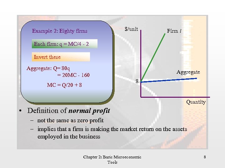
Example 2: Eighty firms $/unit Firm i Each firm: MCMC/4+ 8 q = = 4 q - 2 Invert these Aggregate: Q= 80 q = 20 MC - 160 Aggregate 8 MC = Q/20 + 8 Quantity • Definition of normal profit – not the same as zero profit – implies that a firm is making the market return on the assets employed in the business Chapter 2: Basic Microeconomic Tools 8

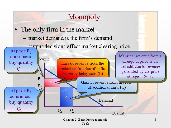
Monopoly • The only firm in the market – market demand is the firm’s demand – output decisions affect market clearing price At price P 1 consumers buy quantity Q 1 $/unit P 1 At price P 2 consumers buy quantity Q 2 P 2 L Marginal revenue from a change in price is the Loss of revenue from the net addition to revenue reduction in price of units generated by the price currently being sold (L) change = G - L Gain in revenue from the sale of additional units (G) G Q 1 Demand Q 2 Chapter 2: Basic Microeconomic Tools Quantity 9

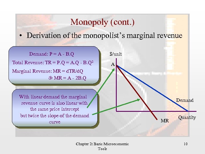
Monopoly (cont. ) • Derivation of the monopolist’s marginal revenue Demand: P = A - B. Q $/unit Total Revenue: TR = P. Q = A. Q - B. Q 2 A Marginal Revenue: MR = d. TR/d. Q MR = A - 2 B. Q With linear demand the marginal revenue curve is also linear with the same price intercept but twice the slope of the demand curve Chapter 2: Basic Microeconomic Tools Demand MR Quantity 10

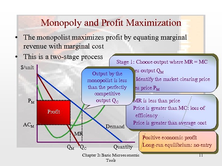
Monopoly and Profit Maximization • The monopolist maximizes profit by equating marginal revenue with marginal cost • This is a two-stage process Stage 1: Choose output where MR = MC $/unit This gives output QM Output by the monopolist is. Stage 2: Identify the market clearing price less MC than the perfectly gives price PM This competitive output QC AC MR is less than price Price is greater than MC: loss of efficiency Price is greater than average cost Demand PM Profit ACM MR QM QC Quantity Chapter 2: Basic Microeconomic Tools Positive economic profit Long-run equilibrium: no entry 11

Profit today versus profit tomorrow • Money today is not the same as money tomorrow – need way to convert tomorrow’s money into today’s – important since firms make decisions over time • is it better to make profit now or invest for future profit? • how should investment in durable assets be judged? – sacrificing profit today imposes a cost • is this cost justified? • Techniques from financial markets can be applied – the concept of discounting and present value Chapter 2: Basic Microeconomic Tools 12

The concept of discounting • Take a simple example: – – – you have $1, 000 this can be deposited in the bank at 5% per annum interest or it can be loaned to a start-up company for one year how much will the start-up have to contract to repay? $1, 000 x (1 + 5/100) = $1, 000 x 1. 05 = $1, 050 • More generally: – you have a sum of money Y – can generate an interest rate r per annum (in the example r = 0. 05) – so it will grow to Y(1 + r) in one year – but then Y today trades for Y(1 + r) in one year’s time Chapter 2: Basic Microeconomic Tools 13

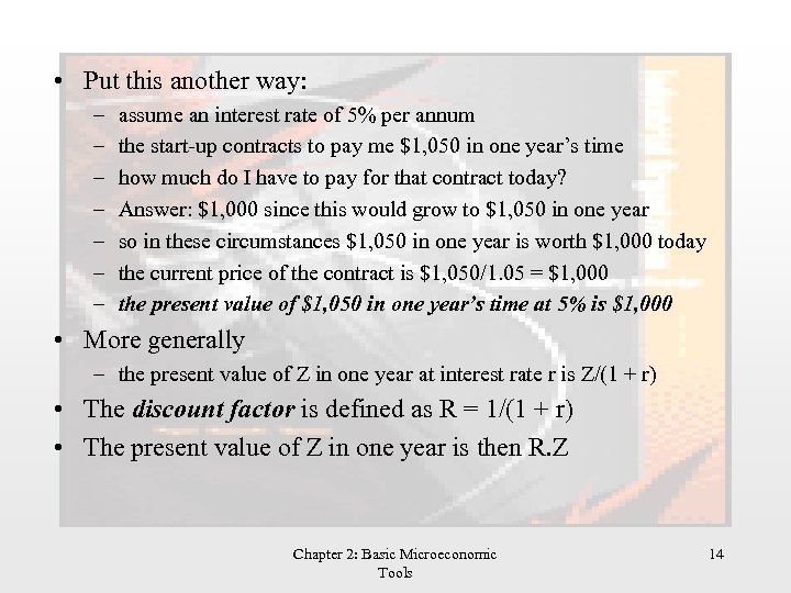
• Put this another way: – – – – assume an interest rate of 5% per annum the start-up contracts to pay me $1, 050 in one year’s time how much do I have to pay for that contract today? Answer: $1, 000 since this would grow to $1, 050 in one year so in these circumstances $1, 050 in one year is worth $1, 000 today the current price of the contract is $1, 050/1. 05 = $1, 000 the present value of $1, 050 in one year’s time at 5% is $1, 000 • More generally – the present value of Z in one year at interest rate r is Z/(1 + r) • The discount factor is defined as R = 1/(1 + r) • The present value of Z in one year is then R. Z Chapter 2: Basic Microeconomic Tools 14

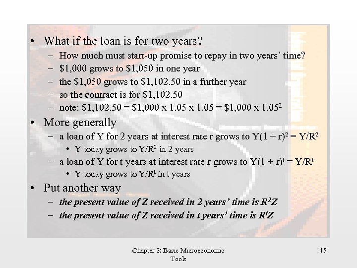
• What if the loan is for two years? – – – How much must start-up promise to repay in two years’ time? $1, 000 grows to $1, 050 in one year the $1, 050 grows to $1, 102. 50 in a further year so the contract is for $1, 102. 50 note: $1, 102. 50 = $1, 000 x 1. 052 • More generally – a loan of Y for 2 years at interest rate r grows to Y(1 + r)2 = Y/R 2 • Y today grows to Y/R 2 in 2 years – a loan of Y for t years at interest rate r grows to Y(1 + r)t = Y/Rt • Y today grows to Y/Rt in t years • Put another way – the present value of Z received in 2 years’ time is R 2 Z – the present value of Z received in t years’ time is Rt. Z Chapter 2: Basic Microeconomic Tools 15

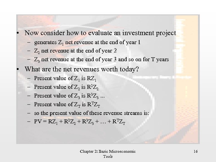
• Now consider how to evaluate an investment project – generates Z 1 net revenue at the end of year 1 – Z 2 net revenue at the end of year 2 – Z 3 net revenue at the end of year 3 and so on for T years • What are the net revenues worth today? – – – Present value of Z 1 is RZ 1 Present value of Z 2 is R 2 Z 2 Present value of Z 3 is R 3 Z 3. . . Present value of ZT is RTZT so the present value of these revenue streams is: PV = RZ 1 + R 2 Z 2 + R 3 Z 3 + … + RTZT Chapter 2: Basic Microeconomic Tools 16

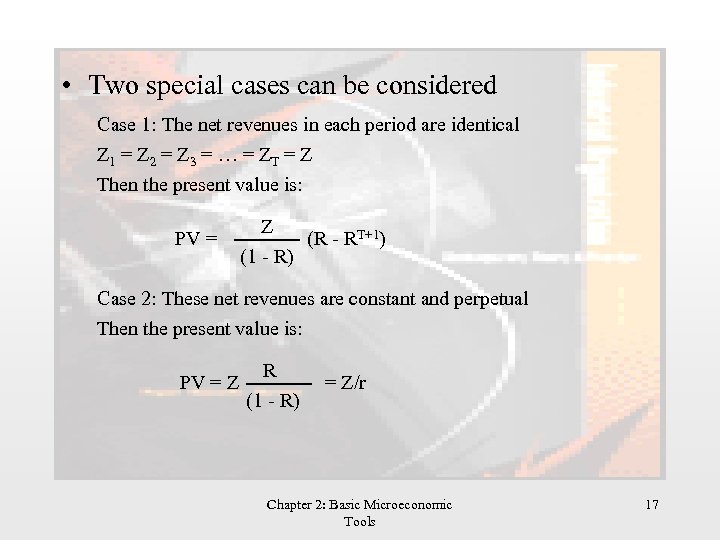
• Two special cases can be considered Case 1: The net revenues in each period are identical Z 1 = Z 2 = Z 3 = … = Z Then the present value is: PV = Z (R - RT+1) (1 - R) Case 2: These net revenues are constant and perpetual Then the present value is: PV = Z R (1 - R) = Z/r Chapter 2: Basic Microeconomic Tools 17

Present value and profit maximization • Present value is directly relevant to profit maximization • For a project to go ahead the rule is – the present value of future income must at least cover the present value of the expenses in establishing the project • The appropriate concept of profit is profit over the lifetime of the project • The application of present value techniques selects the appropriate investment projects that a firm should undertake to maximize its value Chapter 2: Basic Microeconomic Tools 18

Efficiency and Surplus • Can we reallocate resources to make some individuals better off without making others worse off? • Need a measure of well-being – consumer surplus: difference between the maximum amount a consumer is willing to pay for a unit of a good and the amount actually paid for that unit – aggregate consumer surplus is the sum over all units consumed and all consumers – producer surplus: difference between the amount a producer receives from the sale of a unit and the amount that unit costs to produce – aggregate producer surplus is the sum over all units produced and all producers – total surplus = consumer surplus + producer surplus Chapter 2: Basic Microeconomic Tools 19

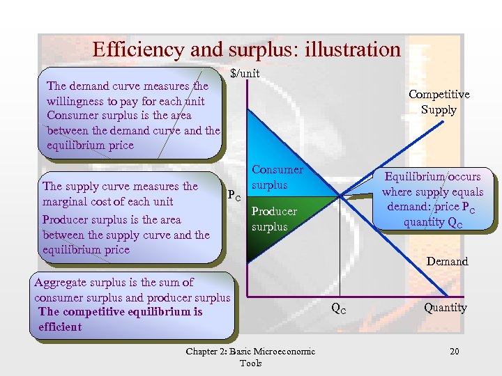
Efficiency and surplus: illustration The demand curve measures the willingness to pay for each unit Consumer surplus is the area between the demand curve and the equilibrium price The supply curve measures the marginal cost of each unit Producer surplus is the area between the supply curve and the equilibrium price $/unit Competitive Supply PC Consumer surplus Equilibrium occurs where supply equals demand: price PC quantity QC Producer surplus Aggregate surplus is the sum of consumer surplus and producer surplus The competitive equilibrium is efficient Chapter 2: Basic Microeconomic Tools Demand QC Quantity 20

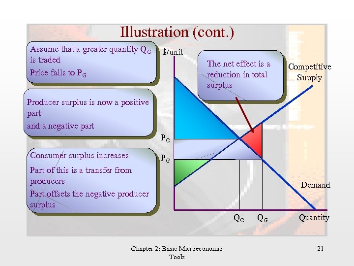
Illustration (cont. ) Assume that a greater quantity QG is traded Price falls to PG $/unit The net effect is a reduction in total surplus Competitive Supply Producer surplus is now a positive part and a negative part PC Consumer surplus increases PG Part of this is a transfer from producers Part offsets the negative producer surplus Demand QC Chapter 2: Basic Microeconomic Tools QG Quantity 21

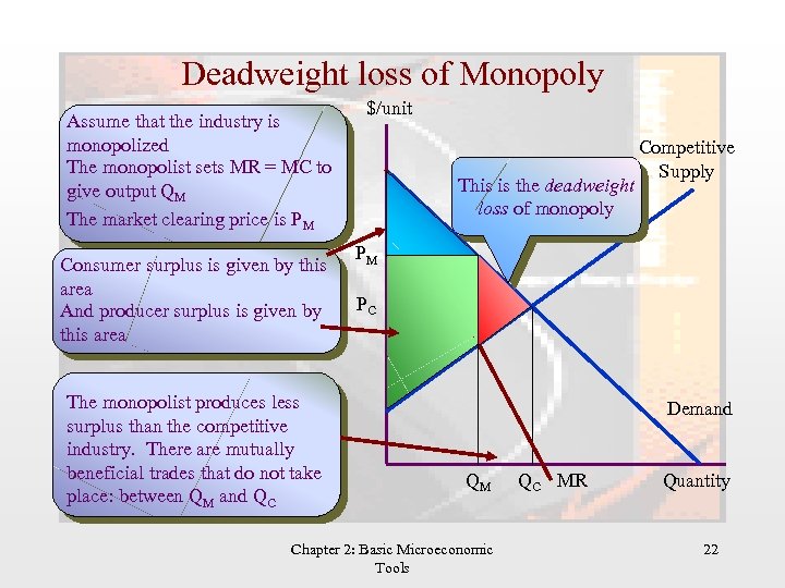
Deadweight loss of Monopoly Assume that the industry is monopolized The monopolist sets MR = MC to give output QM The market clearing price is PM Consumer surplus is given by this area And producer surplus is given by this area The monopolist produces less surplus than the competitive industry. There are mutually beneficial trades that do not take place: between QM and QC $/unit This is the deadweight loss of monopoly Competitive Supply PM PC Demand QM Chapter 2: Basic Microeconomic Tools QC MR Quantity 22

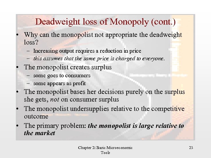
Deadweight loss of Monopoly (cont. ) • Why can the monopolist not appropriate the deadweight loss? – Increasing output requires a reduction in price – this assumes that the same price is charged to everyone. • The monopolist creates surplus – some goes to consumers – some appears as profit • The monopolist bases her decisions purely on the surplus she gets, not on consumer surplus • The monopolist undersupplies relative to the competitive outcome • The primary problem: the monopolist is large relative to the market Chapter 2: Basic Microeconomic Tools 23

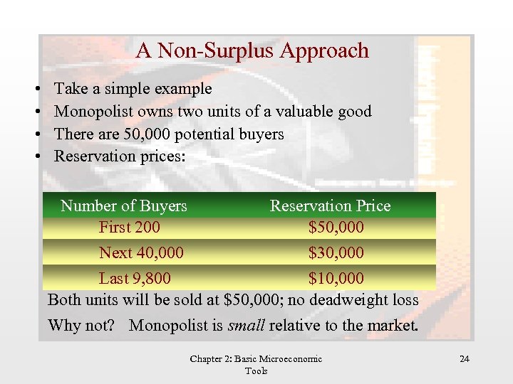
A Non-Surplus Approach • • Take a simple example Monopolist owns two units of a valuable good There are 50, 000 potential buyers Reservation prices: Number of Buyers Reservation Price First 200 $50, 000 Next 40, 000 $30, 000 Last 9, 800 $10, 000 Both units will be sold at $50, 000; no deadweight loss Why not? Monopolist is small relative to the market. Chapter 2: Basic Microeconomic Tools 24

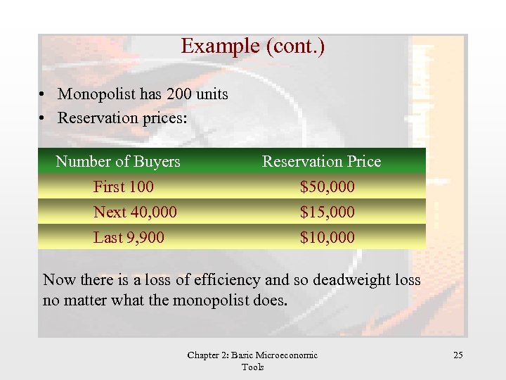
Example (cont. ) • Monopolist has 200 units • Reservation prices: Number of Buyers First 100 Next 40, 000 Last 9, 900 Reservation Price $50, 000 $15, 000 $10, 000 Now there is a loss of efficiency and so deadweight loss no matter what the monopolist does. Chapter 2: Basic Microeconomic Tools 25