b44c17edf5d2e4c8cb5ddabe7704d3c6.ppt
- Количество слайдов: 15
BA 275 Quantitative Business Methods Agenda n Simple Linear Regression n n Inference for Regression Inference for Prediction 1
Regression Analysis n A technique to examine the relationship between an outcome variable (dependent variable, Y) and a group of explanatory variables (independent variables, X 1, X 2, … Xk). n The model allows us to understand (quantify) the effect of each X on Y. n It also allows us to predict Y based on X 1, X 2, …. Xk. 2
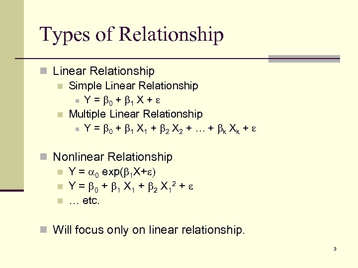
Types of Relationship n Linear Relationship n Simple Linear Relationship n Y = b 0 + b 1 X + e n Multiple Linear Relationship n Y = b 0 + b 1 X 1 + b 2 X 2 + … + bk Xk + e n Nonlinear Relationship n Y = a 0 exp(b 1 X+e) n Y = b 0 + b 1 X 1 + b 2 X 12 + e n … etc. n Will focus only on linear relationship. 3
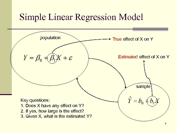
Simple Linear Regression Model population True effect of X on Y Estimated effect of X on Y sample Key questions: 1. Does X have any effect on Y? 2. If yes, how large is the effect? 3. Given X, what is the estimated Y? 4
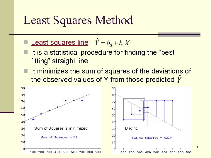
Least Squares Method n Least squares line: n It is a statistical procedure for finding the “best- fitting” straight line. n It minimizes the sum of squares of the deviations of the observed values of Y from those predicted Sum of Squares is minimized. Bad fit. 5
Initial Analysis n Summary statistics + Plots (e. g. , histograms + scatter plots) + Correlations n Things to look for Features of Data (e. g. , data range, outliers) n do not want to extrapolate outside data range because the relationship is unknown (or unestablished). n Summary statistics and graphs. n Is the assumption of linearity appropriate? n 6
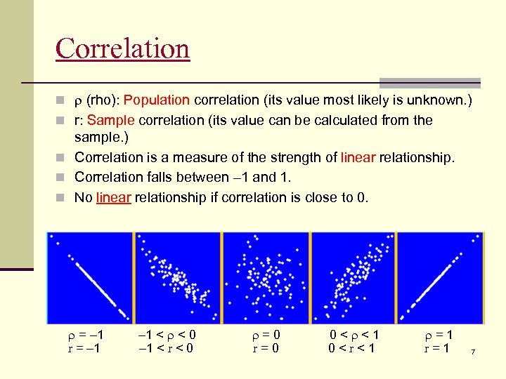
Correlation n r (rho): Population correlation (its value most likely is unknown. ) n r: Sample correlation (its value can be calculated from the sample. ) n Correlation is a measure of the strength of linear relationship. n Correlation falls between – 1 and 1. n No linear relationship if correlation is close to 0. r = – 1 – 1 < r < 0 r=0 0<r<1 r=1 7
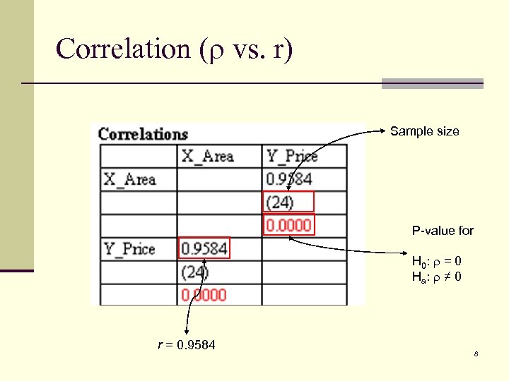
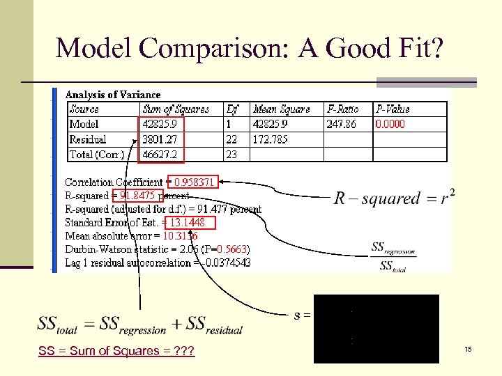
Correlation (r vs. r) Sample size P-value for H 0 : r = 0 Ha : r ≠ 0 r = 0. 9584 8
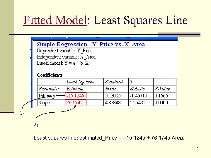
Fitted Model: Least Squares Line b 0 b 1 Least squares line: estimated_Price = – 15. 1245 + 76. 1745 Area. 9
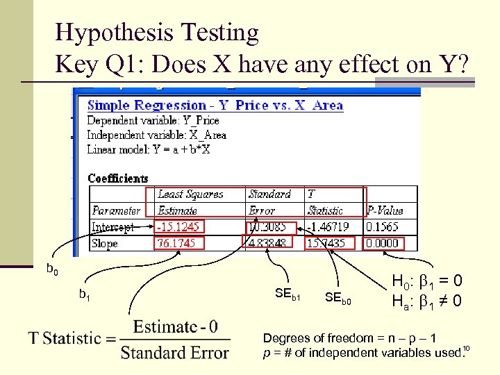
Hypothesis Testing Key Q 1: Does X have any effect on Y? b 0 b 1 SEb 0 H 0: b 1 = 0 H a: b 1 ≠ 0 Degrees of freedom = n – p – 1 10 p = # of independent variables used.
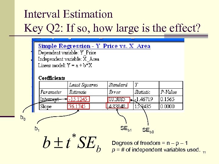
Interval Estimation Key Q 2: If so, how large is the effect? b 0 b 1 SEb 0 Degrees of freedom = n – p – 1 p = # of independent variables used. 11
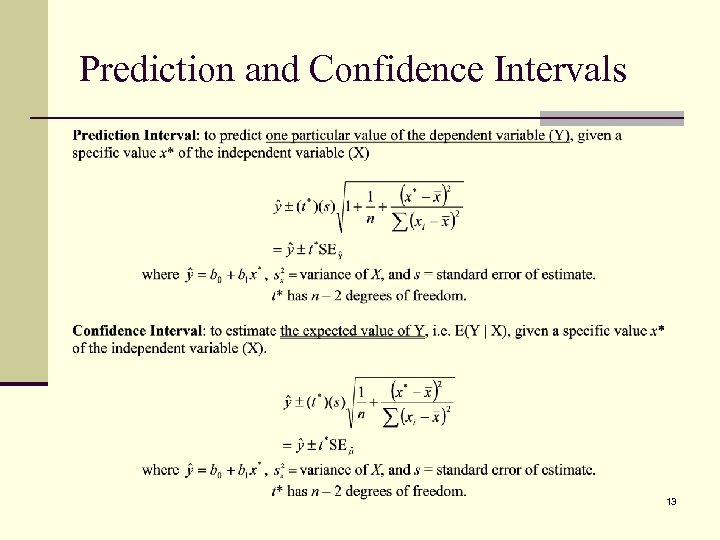
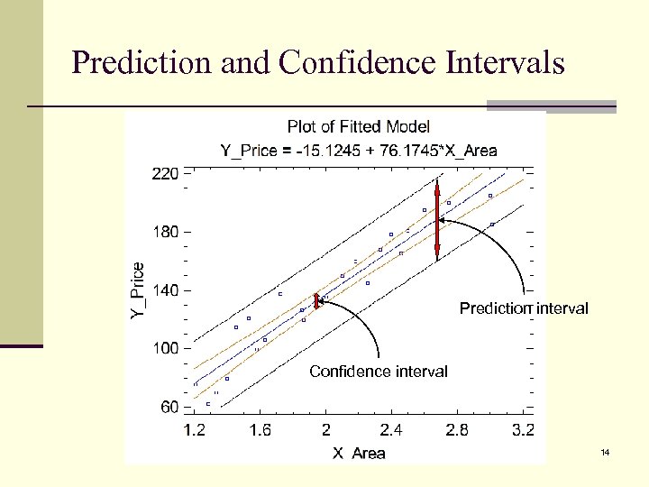
Prediction and Confidence Intervals Key Q 3: Given X, what is the estimated Y? n What is your estimated price of that 2000 -sf house on the 9 th street? n Quick answer: estimated price = -15. 1245 + 76. 1745 (2) = 137. 2245 n What is the average price of a house that occupies 2000 sf? n Quick answer: estimated price = -15. 1245 + 76. 1745 (2) = 137. 2245 n What is the difference? 12
Prediction and Confidence Intervals 13
Prediction and Confidence Intervals Prediction interval Confidence interval 14
Model Comparison: A Good Fit? s= SS = Sum of Squares = ? ? ? 15
b44c17edf5d2e4c8cb5ddabe7704d3c6.ppt