AVMs and CAMA The robots are taking over

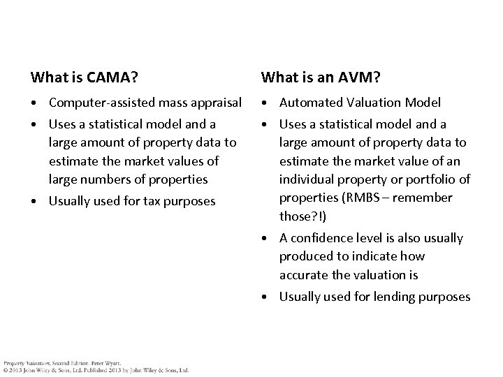
What is CAMA? What is an AVM? • Computer-assisted mass appraisal • Automated Valuation Model • Uses a statistical model and a large amount of property data to estimate the market values of large numbers of properties • Uses a statistical model and a large amount of property data to estimate the market value of an individual property or portfolio of properties (RMBS – remember those? !) • Usually used for tax purposes • A confidence level is also usually produced to indicate how accurate the valuation is • Usually used for lending purposes

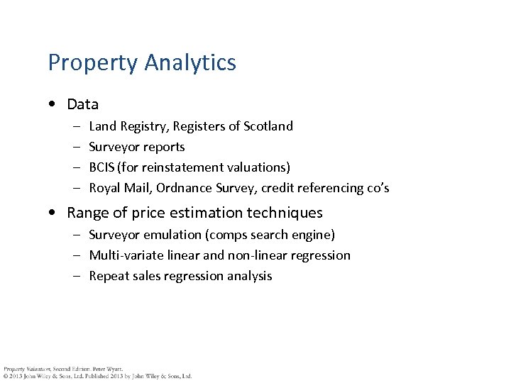
Property Analytics • Data – – Land Registry, Registers of Scotland Surveyor reports BCIS (for reinstatement valuations) Royal Mail, Ordnance Survey, credit referencing co’s • Range of price estimation techniques – Surveyor emulation (comps search engine) – Multi-variate linear and non-linear regression – Repeat sales regression analysis

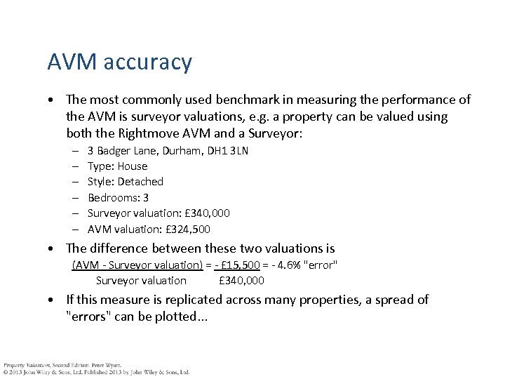
AVM accuracy • The most commonly used benchmark in measuring the performance of the AVM is surveyor valuations, e. g. a property can be valued using both the Rightmove AVM and a Surveyor: – – – 3 Badger Lane, Durham, DH 1 3 LN Type: House Style: Detached Bedrooms: 3 Surveyor valuation: £ 340, 000 AVM valuation: £ 324, 500 • The difference between these two valuations is (AVM - Surveyor valuation) = - £ 15, 500 = - 4. 6% "error" Surveyor valuation £ 340, 000 • If this measure is replicated across many properties, a spread of "errors" can be plotted. . .

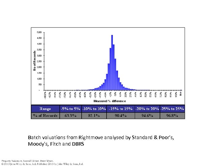
Batch valuations from Rightmove analysed by Standard & Poor's, Moody's, Fitch and DBRS

Statistical model • Use multiple regression analysis (MRA) to infer a mathematical (e. g. linear) relationship between several property attributes and the price that a dwelling might trade for • Property attributes: size, type, age, location, etc. • Mathematical relationship encapsulated in an equation which can be used to estimate price in cases where the attributes are known but the price isn’t

Different from conventional valuation • Relies on large data set – big problem in UK • Provides a valuation and an estimate of variance • Quick • Cheap • Difficult to defend • Difficult to sue an AVM

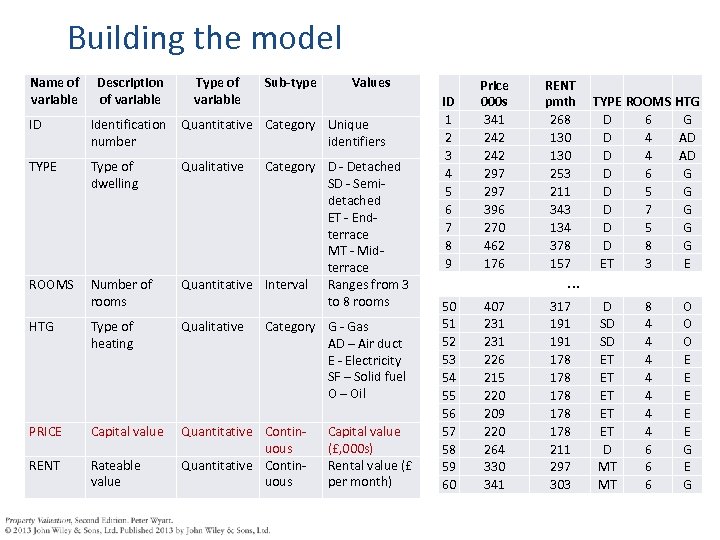
Building the model Name of variable Description of variable Type of variable Sub-type Values ID Identification Quantitative Category Unique number identifiers TYPE Type of dwelling ROOMS Number of rooms Qualitative Category D - Detached SD - Semidetached ET - Endterrace MT - Midterrace Quantitative Interval Ranges from 3 to 8 rooms HTG Type of heating Qualitative Category G - Gas AD – Air duct E - Electricity SF – Solid fuel O – Oil PRICE Capital value RENT Rateable value Quantitative Continuous Capital value (£, 000 s) Rental value (£ per month) ID 1 2 3 4 5 6 7 8 9 Price 000 s 341 242 297 396 270 462 176 RENT pmth 268 130 253 211 343 134 378 157 50 51 52 53 54 55 56 57 58 59 60 407 231 226 215 220 209 220 264 330 341 317 191 178 178 178 211 297 303 . . . TYPE ROOMS HTG D 6 G D 4 AD D 6 G D 5 G D 7 G D 5 G D 8 G ET 3 E D SD SD ET ET ET D MT MT 8 4 4 4 4 6 6 6 O O O E E E G

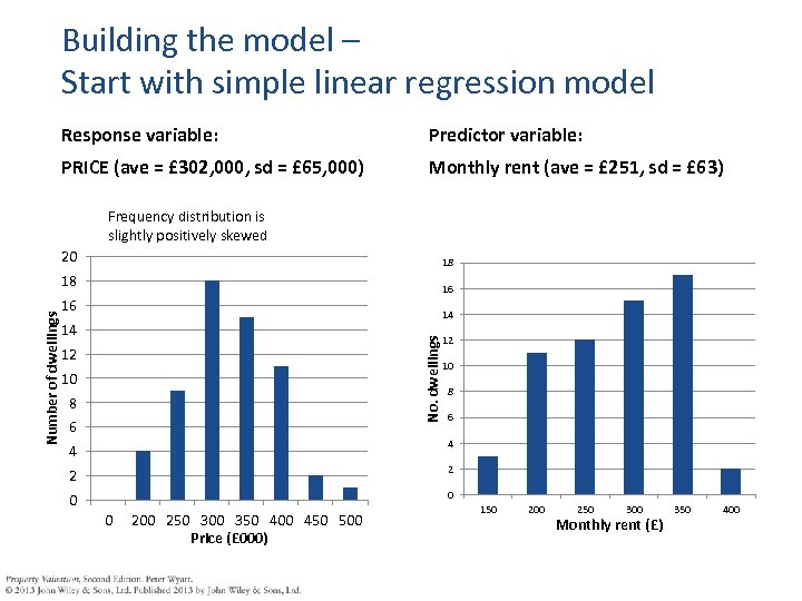
Building the model – Start with simple linear regression model Response variable: Predictor variable: PRICE (ave = £ 302, 000, sd = £ 65, 000) Monthly rent (ave = £ 251, sd = £ 63) Frequency distribution is slightly positively skewed 18 18 16 16 14 14 No. dwellings Number of dwellings 20 12 10 8 6 4 4 2 2 0 0 0 200 250 300 350 400 450 500 Price (£ 000) 150 200 250 300 Monthly rent (£) 350 400

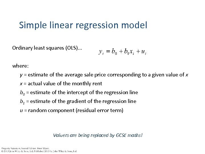
Simple linear regression model Ordinary least squares (OLS). . . where: y = estimate of the average sale price corresponding to a given value of x x = actual value of the monthly rent b 0 = estimate of the intercept of the regression line b 1 = estimate of the gradient of the regression line u = random component (residual error term) Valuers are being replaced by GCSE maths!

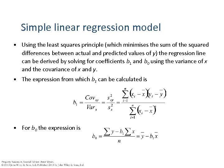
Simple linear regression model • Using the least squares principle (which minimises the sum of the squared differences between actual and predicted values of y) the regression line can be derived by solving for coefficients b 1 and b 0 using the variance of x and the covariance of x and y. • The expression from which b 1 can be calculated is • For b 0 the expression is

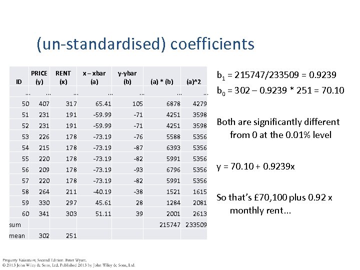
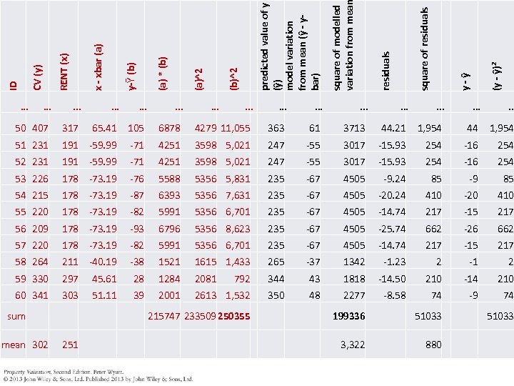
(un-standardised) coefficients PRICE (y) ID RENT (x) x – xbar (a) y-ybar (b) (a) * (b) b 1 = 215747/233509 = 0. 9239 (a)^2 b 0 = 302 – 0. 9239 * 251 = 70. 10 . . 50 407 317 65. 41 105 6878 4279 51 231 191 -59. 99 -71 4251 3598 52 231 191 -59. 99 -71 4251 3598 53 226 178 -73. 19 -76 5588 5356 54 215 178 -73. 19 -87 6393 5356 55 220 178 -73. 19 -82 5991 5356 56 209 178 -73. 19 -93 6796 5356 y = 70. 10 + 0. 9239 x 57 220 178 -73. 19 -82 5991 5356 58 264 211 -40. 19 -38 1521 1615 59 330 297 45. 61 28 1284 2081 60 341 303 51. 11 39 2001 2613 sum mean 215747 233509 302 251 Both are significantly different from 0 at the 0. 01% level So that’s £ 70, 100 plus 0. 92 x monthly rent. . .

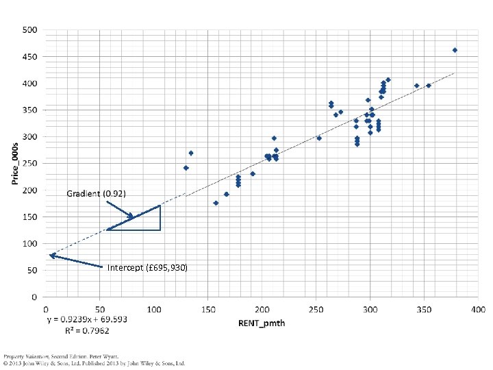
Intercept (£ 695, 930)

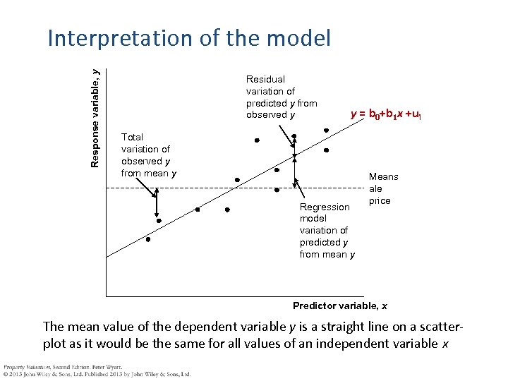
Response variable, y Interpretation of the model Residual variation of predicted y from observed y y = b 0+b 1 x +ui Total variation of observed y from mean y Regression model variation of predicted y from mean y Means ale price Predictor variable, x The mean value of the dependent variable y is a straight line on a scatterplot as it would be the same for all values of an independent variable x

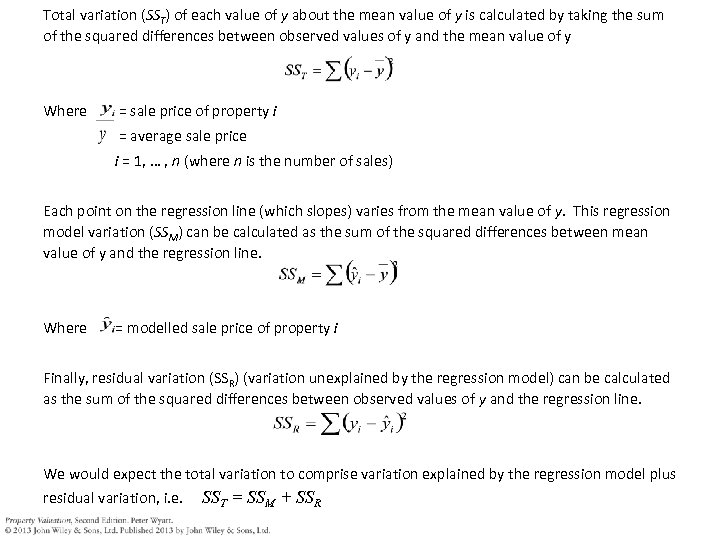
Total variation (SST) of each value of y about the mean value of y is calculated by taking the sum of the squared differences between observed values of y and the mean value of y Where = sale price of property i = average sale price i = 1, … , n (where n is the number of sales) Each point on the regression line (which slopes) varies from the mean value of y. This regression model variation (SSM) can be calculated as the sum of the squared differences between mean value of y and the regression line. Where = modelled sale price of property i Finally, residual variation (SSR) (variation unexplained by the regression model) can be calculated as the sum of the squared differences between observed values of y and the regression line. We would expect the total variation to comprise variation explained by the regression model plus residual variation, i. e. SST = SSM + SSR

. . . . 50 407 317 65. 41 105 51 231 191 -59. 99 52 231 (y - ŷ)2 y - ŷ square of residuals . . . 6878 4279 11, 055 363 61 3713 44. 21 1, 954 44 1, 954 -71 4251 3598 5, 021 247 -55 3017 -15. 93 254 -16 254 191 -59. 99 -71 4251 3598 5, 021 247 -55 3017 -15. 93 254 -16 254 53 226 178 -73. 19 -76 5588 5356 5, 831 235 -67 4505 -9. 24 85 -9 85 54 215 178 -73. 19 -87 6393 5356 7, 631 235 -67 4505 -20. 24 410 -20 410 55 220 178 -73. 19 -82 5991 5356 6, 701 235 -67 4505 -14. 74 217 -15 217 56 209 178 -73. 19 -93 6796 5356 8, 623 235 -67 4505 -25. 74 662 -26 662 57 220 178 -73. 19 -82 5991 5356 6, 701 235 -67 4505 -14. 74 217 -15 217 58 264 211 -40. 19 -38 1521 1615 1, 433 265 -37 1342 -1. 23 2 -1 2 59 330 297 45. 61 28 1284 2081 792 344 43 1818 -14. 50 210 -14 210 60 341 303 51. 11 39 2001 2613 1, 532 350 48 2277 -8. 58 74 -9 74 sum mean 302 . . . square of modelled variation from mea predicted value of y (ŷ) model variation from mean (ŷ - ybar) (b)^2 (a) * (b) y-Ῡ (b) x - xbar (a) RENT (x) CV (y) ID. . . 215747 233509 250355 251 199336 51033 3, 322 880 51033

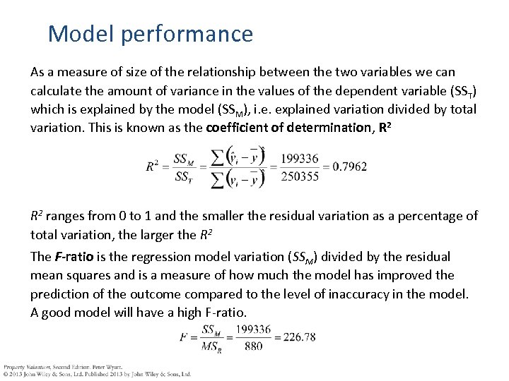
Model performance As a measure of size of the relationship between the two variables we can calculate the amount of variance in the values of the dependent variable (SS T) which is explained by the model (SSM), i. e. explained variation divided by total variation. This is known as the coefficient of determination, R 2 ranges from 0 to 1 and the smaller the residual variation as a percentage of total variation, the larger the R 2 The F-ratio is the regression model variation (SSM) divided by the residual mean squares and is a measure of how much the model has improved the prediction of the outcome compared to the level of inaccuracy in the model. A good model will have a high F-ratio.

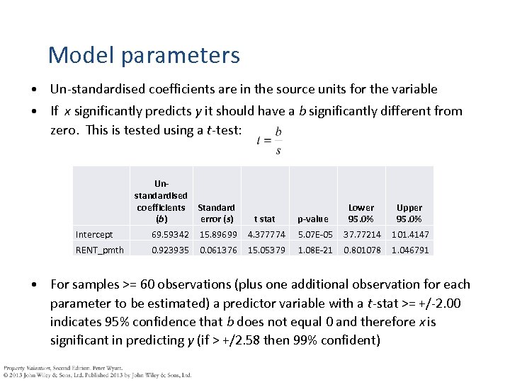
Model parameters • Un-standardised coefficients are in the source units for the variable • If x significantly predicts y it should have a b significantly different from zero. This is tested using a t-test: Unstandardised coefficients Standard (b) error (s) t stat p-value Lower 95. 0% Upper 95. 0% Intercept 69. 59342 15. 89699 4. 377774 5. 07 E-05 37. 77214 101. 4147 RENT_pmth 0. 923935 0. 061376 15. 05379 1. 08 E-21 0. 801078 1. 046791 • For samples >= 60 observations (plus one additional observation for each parameter to be estimated) a predictor variable with a t-stat >= +/-2. 00 indicates 95% confidence that b does not equal 0 and therefore x is significant in predicting y (if > +/2. 58 then 99% confident)

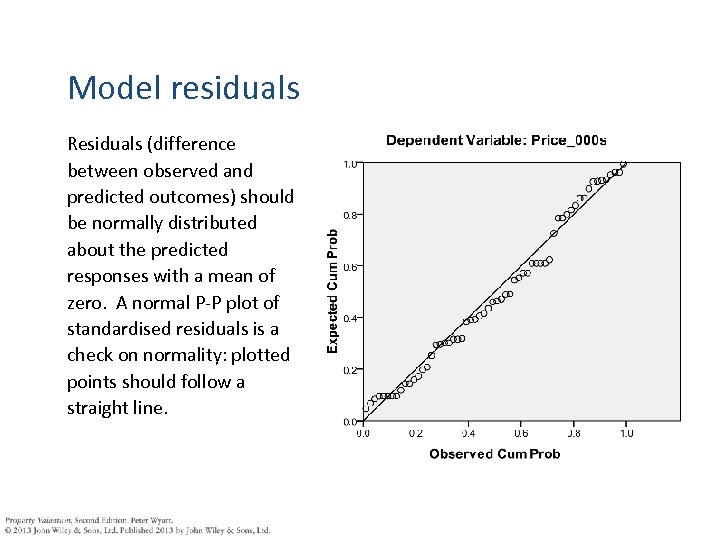
Model residuals Residuals (difference between observed and predicted outcomes) should be normally distributed about the predicted responses with a mean of zero. A normal P-P plot of standardised residuals is a check on normality: plotted points should follow a straight line.

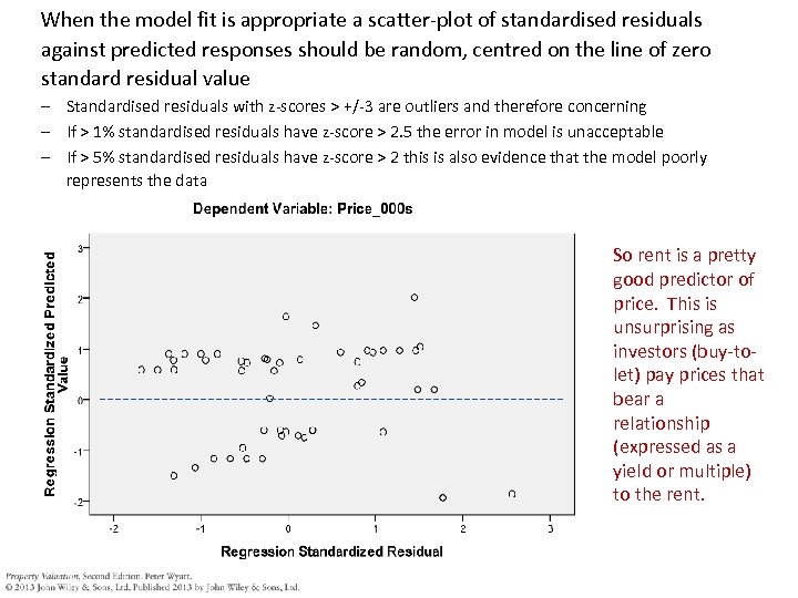
When the model fit is appropriate a scatter-plot of standardised residuals against predicted responses should be random, centred on the line of zero standard residual value – Standardised residuals with z-scores > +/-3 are outliers and therefore concerning – If > 1% standardised residuals have z-score > 2. 5 the error in model is unacceptable – If > 5% standardised residuals have z-score > 2 this is also evidence that the model poorly represents the data So rent is a pretty good predictor of price. This is unsurprising as investors (buy-tolet) pay prices that bear a relationship (expressed as a yield or multiple) to the rent.