Aviation Mesoscale Numerical Weather Prediction by George A

Aviation Mesoscale Numerical Weather Prediction by George A. Isaac Weather Impacts Consulting Incorporated WMO WWRP & CAe. M Aviation Research Demonstration Project (Av. RDP) Training Workshop , 20 -22 July 2016, Hong Kong

Introduction • Weather related accidents

Introduction cont. • According to Boeing most accidents occur during landing and take off

Mesoscale Models • Usually initialized using larger scale models. • Now routinely have several km resolution with 100 s of meters possible. • Need high time resolution. • Required for airport applications because many variables are sensitive to local terrain (hills, lakes, ocean, etc). • Boundary layer issues remain a big problem. Most of issues occur in boundary layer, low ceilings, visibility, severe winds, etc. • Generally not good for convection/lightning.

Mesoscale Models (cont. . ) • Modelling community tends not to verify their mesoscale models for aviation related variables. • Verification for rare events is very difficult. • Need to know the limitations of the models. • Trend is towards more automation using models (e. g. auto. TAF) but this might be premature. • Forecasters are still required to interpret the model outputs.

Mesoscale Models … cont. • There are many mesoscale models available to the aviation user. If possible, it would be good to use more than one. Strangely enough, intuition regarding which model would be best can be wrong. Are models with highest resolution better? Does more levels in the boundary layer help? Are models with “rapid update cycles” superior? Does radar data assimilation help? Etc. Again, there is a need to verify each model to learn its strengths and weaknesses. However, they are typically updated often which means that verification statistics can be out-of-date.

Mesoscale Models…. cont • Some forecasters tend not to believe model results because they are often wrong. But they fail to realize that the human forecaster is also often wrong. • Alister Ling, a Senior Aviation Meteorologist at ECCC, tells relative newcomers that “you’re a fool to accept the model without checking and you’re an idiot if you reject it as inferior to your skill. ”

How to Forecast? • Precipitation Types, Visibility, Ceiling, Precipitation Amount, Convection, Blowing Snow, Lightning, Aircraft Icing, Turbulence, Wind Shear • What is more important? Enroute forecasting to avoid congestion or forecasting at airport itself? • (How do you do it now? ? Do you use a Model? )

Terminal Area Forecasts • Terminal Area Forecasts are now handled by TAFs which are old technology and don’t convey all the information needed. • However, ECCC, like other organizations, are working on auto. TAF in which TAFs are created directly from model output. • What follows are some comments from Alister Ling, a Senior Aviation Meteorologist involved in the development. • Quotes from Alister Ling: • Expect savings only when there is a lot of TAFs with good weather • If you have 3 TAFs with good weather, faster to do it manually!

How green are the official TAFs? • GREEN: The *entire* TAF had no MVFR, no PROB TS/FG • RED: IFR at some point in the TAF • Note strong day-to-day variability; difficult to schedule desk reductions ahead of time • poor late autumn-winter wx • Potential gains in spring and just before autumn turns cold From A. Ling, ECCC

If the model is “wrong”, so too the auto. TAF • Sites with great topographic variability and strong local effects (see below) • When close to a stratus edge • Patchy boundary layer Misses very light precip (-SN FG or -SN IC or DZ/FZDZ/SG) • Beyond 12 h of the nowcast, the system cannot differentiate between -DZ and –RA • Mountain-valley funneling and cold pools • Disorganized convection (misses, or with a hit takes vis too low) • Nowcast can be inconsistent with models - over-rules model in first 12 h • Misses CU/SC/TCU of 1 -5 oktas • Lake effect snowsqualls • Lake/land breezes missed by UMOS • Advection marine stratus can be tricky • Cannot forecast obscuration: HZ, IC, FU, VA, BLDU, BLSN • LLJ over cold surface: model too stable, misses gusts and pumping winds • Cig/Vis goes to zero [but corrected with climate values when available] in continuous precip From A. Ling, ECCC

Continued … • Cold stable, humid airmass (arctic airmass) • misses IC, over-forecasts OVC 000 and 0 SM • Fog model is simplistic (partially compensated by ACC climatology) • Vis too low in isolated shower because it assumes rain is homogeneous out to 15 km (uses Marshall-Palmer relation to droplet size which affects vis). • CB base unreasonably low at times. • CB PROB values are to be used only as a flag. It is PROB 30 even if the underlying data says PROB 80. • CB vis and gust are simplistic (constants modified by values in the MAIN condition) • Gust “turns off” too early in the evening, too light in cold FROPA From A. Ling, ECCC

Wind Shear (Emily Zhou, MSc Thesis York U. ) From AMDAR, wind shear cases occur more often in autumn and winter, and during local morning. 70% of wind shear cases are present at 1 st 500 ft. REG, LAM and RUC are not capable of forecasting low level wind shear directly for Pearson Airport. Wind Shear Threshold at 500 ft is 25 kts or 12. 9 m/s.

SNOW-V 10 Science of Nowcasting Olympic Weather for Vancouver 2010 A World Weather Research Programme approved project • To improve our understanding and ability to forecast/nowcast low cloud, and visibility. • To improve our understanding and ability to forecast precipitation amount and type. • To improve forecasts of wind speed, gusts and direction. • To develop better forecast production systems. • Assess and evaluate value to end users. • To increase the capacity of WMO member states. Isaac, G. A. , P. Joe, J. Mailhot, M. Bailey, S. Bélair, F. S. Boudala, M. Brugman, E. Campos, R. L. Carpenter Jr. , R. W. Crawford, S. G. Cober, B. Denis, C. Doyle, H. D. Reeves, I. Gultepe, T. Haiden, I. Heckman, L. X. Huang, J. A. Milbrandt, R. Mo, R. M. Rasmussen, T. Smith, R. E. Stewart, D. Wang and L. J. Wilson, 2014: Science of Nowcasting Olympic Weather for Vancouver 2010 (SNOW-10): A World Weather Research Programme project. Pure Appl. Geophys. 171, 1– 24, (DOI: 10. 1007/s 00024 -012 -0579 -0).

Two clusters of «Sochi-2014» Olympic venues Snow sports competitions FROST-2014: Forecast and Research in the Olympic Sochi Testbed Ice sports competitions

Slide from Dmitry Kiktev of Roshydromet, PI of FROST-2014

On-Site Sfc Measurements Observer Reports Radar Data Canadian Airport Nowcasting Forecast System (CAN-Now) Forecaster Input TAF+, Blog On-Site Remote Sensing Microwave Radiometer Vertically Pointing Radar NWP Models GEM REG, GEM LAM, RUC Scientific Algorithms Visibility, RVR, Ceiling, Gust, Precip, Wind Shear, Turbulence, Cross-Winds, AAR, CAT Level, etc. Satellite Data Lightning Data Aircraft Data Pilot Reports Climatology Data Nowcasting Methods ABOM, INTW, Raw NWP, Radar & Lightning Forecast, Conditional Climatology Integrated Forecast and Warning Product (Situation Chart) Spatial Products for Specific Users Web-based Delivery System Time Series Products for Specific Users Real-time Verification Products Terminal Area Forecasts Isaac, G. A. , M, Bailey, F. S. Boudala, W. R. Burrows, S. G. Cober, R. W. Crawford, N. Donaldson, I. Gultepe, B. Hansen, I. Heckman, L. X Huang, A. Ling, J. Mailhot, J. A. Milbrandt, J. Reid, and M. Fournier, 2014: The Canadian airport nowcasting system (CAN-Now). Meteorol. Appl. 21, 30– 49, (DOI: 10. 1002/met. 1342).

Model Resolution From Kiktev et al. , 2016: FROST 2014: the Sochi Winter Olympics International Project. Submitted to BAMS

Model Resolution 2 From Kiktev et al. , 2016: FROST 2014: the Sochi Winter Olympics International Project. Submitted to BAMS

Fog event missed during FROST 2014 (February 17, 2014) by both model scheme used during SNOW -V 10 and diagnostic method of Boudala et al. (2012) using Nowcast RH. Model failed to produce cloud at low levels. The model visibility scheme is descrbed in Gultepe and Milbrandt (2010). Gultepe I, Milbrandt JA. 2010: Probabilistic parameterizations of visibility using observations of rain precipitation rate, relative humidity, and visibility. J. Appl. Meteorol. Climatol. 49: 36– 46.

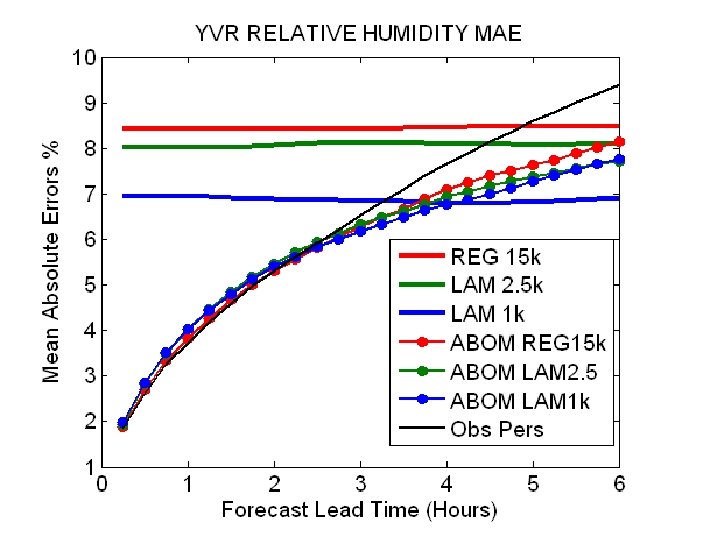
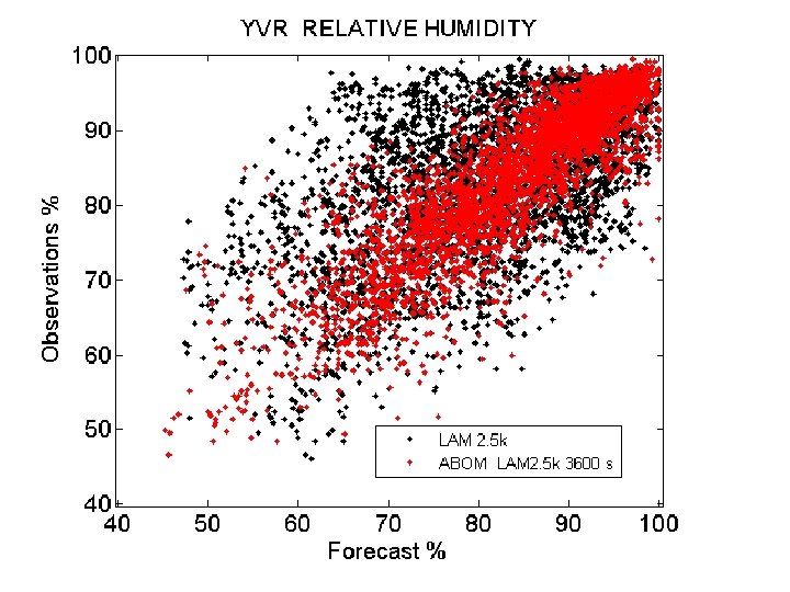
Adaptive Blending of Observations and Model (ABOM): What is it how does it work • • Statistical method for generating point forecasts using model and observation data The current observation + a weighted combination of forecasts from three different methods: 1) Extrapolation of the current observation trend 2) The change predicted by a model forecast 3) Observation persistence • The weights are determined from recent history and are updated every 15 minutes with new observation data (an hour was used in the studies here)

ABOM Forecast at lead time p Current Observation Change predicted by obs trend Change predicted by model • Coefficients s and r are proportional to the performance over recent history, relative to obs persistence (w) and to • • Local tuning parameters (not yet optimized at all SNOWV 10 sites) Updated using new obs data every 15 minutes ABOM reduces to: • Observation persistence when r = s = 0, w = 1 • Pure observation trend when r = 0, s = 1, w = 0 • Model + obs trend + persistence for all other r, s and w

Temperature Mean Absolute Error: Averaged by Nowcast Lead Time to 6 Hours 1) Nowcast - Model crossover lead-time 2) Improvement over persistence

Background of INTW • INTW refers to integrated weighted model • Available models are used to generate INTW • Major steps of INTW generation • Data pre-checking - defining the available NWP models and observations • Extracting the available data for specific variable and location • Calculating statistics from NWP model data, e. g. MAE, RMSE • Deriving weights from model variables based on model performance • Defining and performing dynamic and variational bias correction • Generating Integrated Model forecasts (INTW)

MAE of temperature by SNOW-V 10 site MAE variances INTW: 0. 82 ~ 1. 15 LAM 1 K: 1. 15 ~ 2. 23 LAM 2. 5 K: 1. 19 ~ 2. 05 REG: 1. 20 ~ 4. 15

MAE of relative humidity by lead time INTW has largest MAE at INTW has smallest MAE at Cypress Bowl Callaghan Valley (VOD) North (VOE)

FROST-14 Results

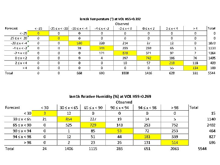
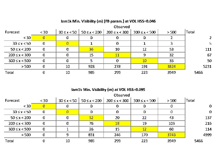
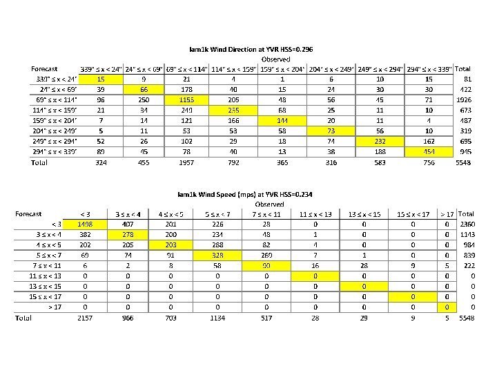
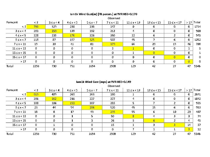
Multi-Categories: HSS and ACC Using: i j Observed category 1 2 3 . . . K total 1 Forecast Category N(F 1) 2 N(F 2) 3 N(F 3) . . N(Fk) K total N(O 1) N(O 2) N(O 3) N(Ok) N

Heidke Skill Score (HSS) answers question “What was the accuracy of the forecast in predicting the correct category, relative to that of random chance? ’ with 1 indicating a perfect score and 0 no skill: The Accuracy Score (ACC) score answers the question ‘Overall, what fraction of the forecasts were in the correct category? ’ with 1 indicating a perfect score and 0 no skill

Categories Used in CAN-Now Analysis

Categories for SNOW-V 10 Analysis

End User Requirements Threshold Matrix for Downhill, Slalom and Giant Slalom (from Chris Doyle) New Snow (24 hours) Wind Visibility Rain Critical Decision point > 30 cm Constant above 17 m/s or gusts > 17 m/s < 200 m on the entire course. Lower Thresholds for GS…course dependant but ~ 100 m for GS 15 mm in 6 hours or less Significant decision point Ø 15 cm and < 30 cm >10 cm and < 30 cm Paralympics) Constant 11 m/s to 17 m/s < 200 m on portions of the course Mixed precipitation Factor to consider > 5 cm > 2 cm within 6 h of an event Gusts above 14 >200 m but <500 m on m/s but < 17 whole or part of the m/s> course

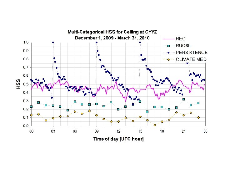
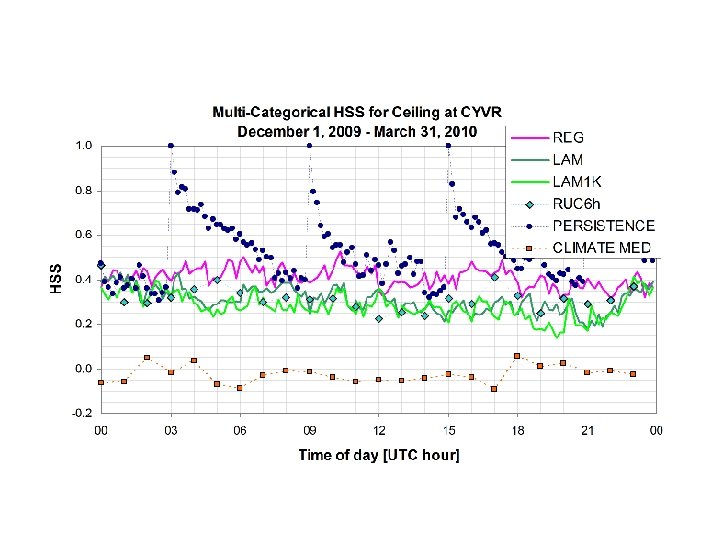
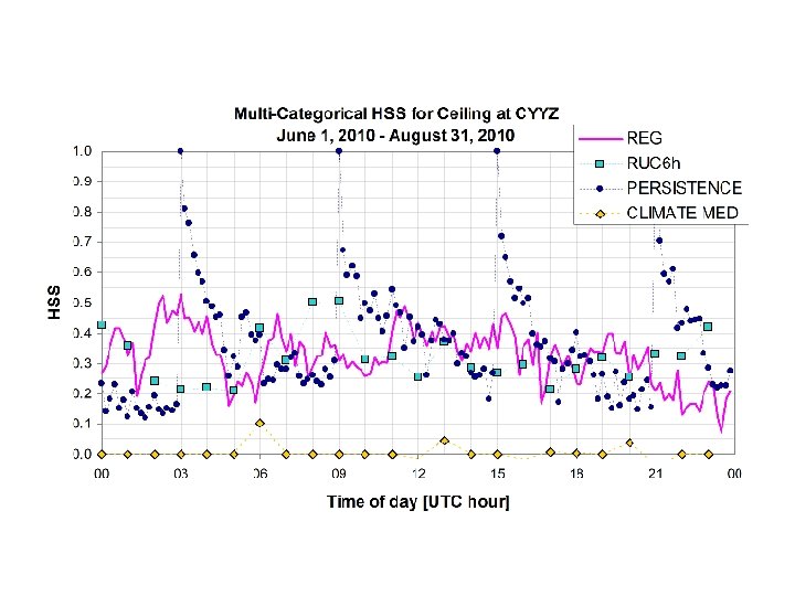
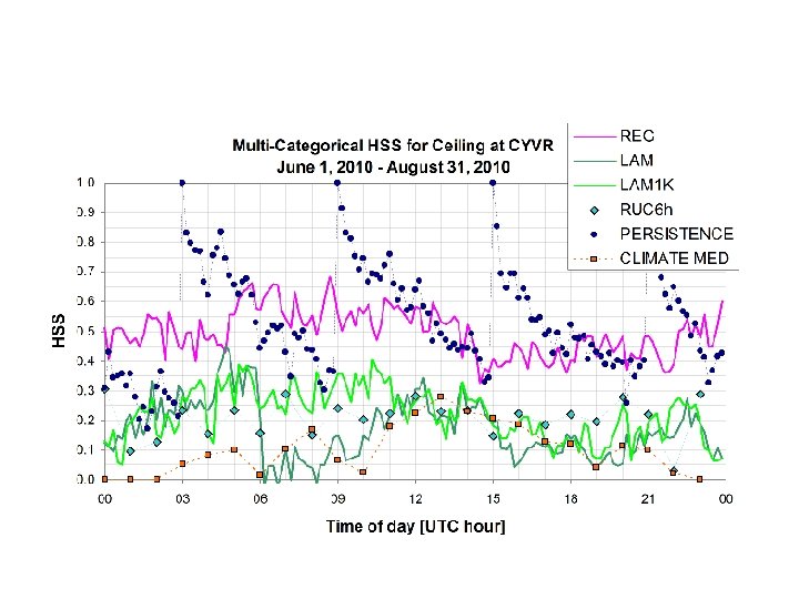
CYYZ Winter CYYZ Summer Relaxed M-C HSS / ACC Ceiling 0. 45 / 0. 62 0. 46 / 0. 61 0. 36 / 063 0. 30 / 0. 55 0. 30 / 0. 70 0. 26 / 0. 62 0. 23 / 0. 86 0. 19 / 0. 78 0. 28 / 0. 78 0. 27 / 0. 70 0. 15 / 0. 78 0. 16 / 0. 73 Precipitation Rate 0. 29 / 0. 73 0. 27 / 0. 67 0. 18 / 0. 91 0. 18 / 0. 85 0. 24 / 0. 75 0. 25 / 0. 71 0. 08 / 0. 80 0. 11 / 0. 77 Ceiling 0. 24 / 0. 47 0. 25 / 0. 45 0. 33 / 0. 67 0. 33 / 0. 63 Precipitation Rate 0. 40 / 0. 84 0. 40 / 0. 81 0. 18 / 0. 90 0. 18 / 0. 85 Visibility RUC 6 h Original M-C HSS / ACC Visibility (BI 09) LAM Relaxed M-C HSS / ACC Visibility (BI 09) REG Original M-C HSS / ACC Precipitation Rate Model 0. 22 / 0. 66 0. 19 / 0. 60 0. 16 / 0. 74 0. 15 / 0. 70 Variable For the original HSS and ACC scores the model data and observations have to match exactly in time. The analysis was redone by looking for the minimum (maximum) model value in ± 60 min of the observed time. For example, minimum visibility or cloud base height, and maximum precipitation rate were selected for the widened period. The results are shown above. The changes to HSS and ACC scores are small and not consistently for the better or worse. (see Isaac et al. (2014))

Can the Forecaster do better than the models in forecasting RH? It appears difficult to beat persistence in the short term although INTW is doing OK. (see Isaac et al. (2014).

Conclusions • Models are currently underused in forecasting aviation weather. • Much more work is necessary in order to use their full potential. • Although they have many problems, they do represent the future. Verification is necessary. • It is useful to combine model output into decision making processes. • Forecasters are essential in the process, to interpret the model output, to notice errors, and to add value.