Autômatos Celulares Disciplina SER 301 Análise Espacial de

Autômatos Celulares Disciplina SER 301 Análise Espacial de Dados Geográficos Líliam C. Castro Medeiros lccastro@dpi. inpe. br Raian Vargas Maretto raian@dpi. inpe. br

Como representar computacionalmente fenômenos geográficos?

Como representar computacionalmente fenômenos geográficos? Itaituba – PA (1985). TM/Landsat-5 composition R(3) G(2) B(1). Source: INPE image catalog Escala temporal? Source: Fred Ramos

Como representar computacionalmente fenômenos geográficos? Fonte: PRODES/INPE Modelos baseados em

Cellular Automata § Dynamic and self -reproducing sistems § Discrete space and time § The basic elements: cells The nth iteration Neumann JV, Burks AW (1966). Theory of Self-Reproducing Automata, University of Illinois Press, Urbana

§ Dynamic and self -reproducing sistems § Discrete space and time § The basic elements: cells The nth iteration Neumann JV, Burks AW (1966). Theory of Self-Reproducing Automata, University of Illinois Press, Urbana

Each cell contains: § A finite set of predeterminated states § A set of transition rules (to change the states) which depend on the cell’s neighborhood The nth iteration Neumann JV, Burks AW (1966). Theory of Self-Reproducing Automata, University of Illinois Press, Urbana

13 Source: Rita Zorzenon’s slide

The Cellular Automata Desenvolvido pelo matemático húngaro John von Neumann, que na década de 40, propôs um modelo baseado na ideia de sistemas lógicos que fossem auto-reprodutores e que imitassem a própria vida. Cooper NG (1983). From Turing and von Neumann to the present. Los Alamos Science.

Source: Carneiro, 2006 Ex: Attribute Land Use: f (It) f (It+1) F F f (It+2) Possible States: • Forested • Agriculture • Urban f ( It+n ) . . . Transition rule based an modeler defined function Source: Gilberto Câmara. 15

Dynamic Spatial Models Forecast tp - 20 tp - 10 tp Calibration Source: Cláudia Almeida Calibration tp + 10

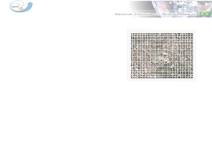
An Example: John Conway’s Game of Life § a regular grid with square cells

An Example: John Conway’s Game of Life § each cell can be white (alive) or black (dead)

An Example: John Conway’s Game of Life § each cell can be white (alive) or black (dead) § for each cell, their neighbors are the 8 closer cells Figure: Leonardo Santos et al. (2011). A susceptible-infected model for exploring the effects of neighborhood structures on epidemic processes – a segregation analysis. Proceedings XII GEOINFO, November 27 -29, 2011, Campos do Jordão, Brazil. p 85 -96.

An Example: John Conway’s Game of Life § each cell can be white (alive) or black (dead) § for each cell, their neighbors are the 8 closer cells § at each time step, the state of each cell obey the following rules (executed simultaneously): § the cell survives if there are 2 or 3 alive neighbor cells, otherwise the cell dies § a died cell can change to an alive cell if it has exatly 3 alive neighbors, otherwise it remains dead

Game of Life John Conway (1970) Possible states: alive or dead Death: by loneliness - one or zero neighbors by overpopulation – more than 4 neighbors Birth: cells with exactly 3 alive neighbors Survival: exactly 2 or exactly 3 alive neighbors Adapted from Adriana Racco’s slide

Rita Zorzenon’s slide 22

Mas a saída são só essas figurinhas? Não consigo ver a coisa acontecendo? 23

Game of Life Some sites to see the Game of Life simulation: http: //www. terrame. org/doku. php? id=examples http: //www. math. com/students/wonders/life. html http: //www. bitstorm. org/gameoflife/

CA = (G, N, S, IC, R, BC, UC) G: Geometry N: Neighborhood S: States IC: Initial condition R: Rules BC: Boundary conditions UC: Updating criteria The CA Structure Source: Adapted from Leonardo Santos’ slide

The Grid

CA = (G, N, S, IC, R, BC, UC) G: Geometry N: Neighborhood S: States IC: Initial condition R: Rules BC: Boundary conditions UC: Updating criteria The CA Structure Source: Adapted from Leonardo Santos’ slide

The Geometry Example: Two-Dimensional Grids with regular Cells that have a common edge with the involved are named as “main neighbors” of the cell (are showed with hatching) The set of actual neighbors of the cell a, which can be found according to N, is denoted as N(a) Source: Lev Naumov’ slide

Irregular Spaces Cell Polygons Lines Points 29

CA = (G, N, S, IC, R, BC, UC) G: Geometry N: Neighborhood S: States IC: Initial condition R: Rules BC: Boundary conditions UC: Updating criteria The CA Structure Adapted from Leonardo Santos’ slide

Vizinhanças Componente essencial nos modelos baseados em AC • Determinam como os elementos do modelo interagem entre si • Duas células são vizinhas se uma exerce alguma influência sobre o estado da outra Fonte Slide: Adaptado de Maretto, 2011 Fonte Fig. : (ANDRADE-NETO et al. , 2008)

Von Neumann Neighborhood First neighbors Second neighbors 32 Adapted from Adriana Racco’s slide

Moore Neighborhood First neighbors Second neighbors 33 Adapted from Adriana Racco’s slide

Random Neighborhood 34 Adapted from Adriana Racco’s slide

Other Neighborhoods The arbitrary neighborhood is determined by the model Examples: First neighbors Second neighbors Based on people activity-space (Santos et al, 2011) Adapted from Adriana Racco’s slide Based on data (Aguiar et al, 2003)

Neighborhoods in Time They can be § static: the same neighbors all the time (classical CA) § dynamic: the neighbors can change at each time step

Neighborhoods in Time Rondônia - 1986 Rondônia 1975 Ocupação Humana [Câmara et al. , 2009]

Neighborhoods in Time Source: Adapted from Maretto, 2011

CA = (G, N, S, IC, R, BC, UC) G: Geometry N: Neighborhood S: States IC: Initial condition R: Rules BC: Boundary conditions UC: Updating criteria The CA Structure Source: Adapted from Leonardo Santos’ slide

Rules § The rules may depend on the state of the own cell neighbor’s cells § The rules may be based on influence fields of the geography of the system § They may be deterministic or stochastic § They can depend only on the actual state of the cells Adapted from Adriana Racco’s slide

CA = (G, N, S, IC, R, BC, UC) G: Geometry N: Neighborhood S: States IC: Initial condition R: Rules BC: Boundary conditions UC: Updating criteria The CA Structure Source: Adapted from Leonardo Santos’ slide

Boundary Conditions § Periodic (1 D - ring or 2 D – torus) 45

Boundary Conditions § Periodic (1 D - ring or 2 D – torus) 46

Boundary Conditions § Periodic (1 D - ring or 2 D – torus) 47

Boundary Conditions § Periodic (1 D - ring or 2 D – torus) 48

Boundary Conditions § Periodic (1 D - ring § Reflexive or 2 D – torus)

Boundary Conditions § Periodic (1 D - ring § Reflexive § Fixed or 2 D – torus)

Boundary Conditions § Periodic (1 D - ring or 2 D – torus) § Reflexive § Fixed § Null (the cells located on the borders have as neighbors only those cells immediately adjacent to them into the grid) § Others

CA = (G, N, S, IC, R, BC, UC) G: Geometry N: Neighborhood S: States IC: Initial condition R: Rules BC: Boundary conditions UC: Updating criteria The CA Structure Source: Adapted from Leonardo Santos’ slide

Examples of Bidimensional Cellular Automata Models

Dengue Fever It is a viral disease trasmitted in Brazil mainly by Aedes aegypti mosquito

Stages of Infection In Mosquitoes Susceptible Infected time Extrinsic Incubation Mosquito infects humans Period Moment of infection 8 to 12 days Figure: Whitehead SS, Blaney JE, Durbin AP, Murphy BR (2007). Prospects for a dengue virus vaccine. Nature Reviews Microbiology, 5: 518 -528.

Dengue Stages In Humans Susceptible Infected Recovered time Intrinsic Contagious Incubation Period Moment of Human infection infects mosquitoes 3 to 14 days Average between 4 and 5 days 4 and 7 days Figure: Whitehead SS, Blaney JE, Durbin AP, Murphy BR (2007). Prospects for a dengue virus vaccine. Nature Reviews Microbiology, 5: 518 -528.

Dengue Virus There are four distinct serotypes of the virus: DENV 1, DENV 2, DENV 3 e DENV 4

The Model

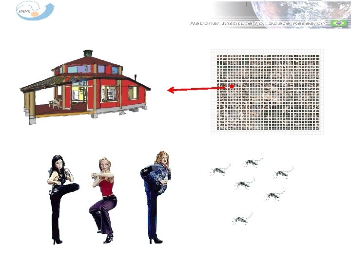
Humans Mosquitoes A multi-level stochastic cellular automata

The Model Humans Mosquitoes

The Model State Time of infection (days) Humans Mosquitoes

The Model Humans Mosquitoes

The Model Humans Mosquitoes Age Time of infection days (days)

Model Considerations § § § Human mobility Asymptomatic people Human renewal House infestation Vector density per household Each iteration corresponds to a day

CA = (G, N, S, IC, R, BC, UC) G: Geometry N: Neighborhood S: States IC: Initial condition R: Rules BC: Boundary conditions UC: Updating criteria The CA Structure Source: Adapted from Leonardo Santos’ slide

CA = (G, N, S, IC, R, BC, UC) Humans G: Geometry N: Neighborhood S: States IC: Initial condition R: Rules BC: Boundary conditions UC: Updating criteria The CA Structure Source: Adapted from Leonardo Santos’ slide Mosquitoes

CA = (G, N, S, IC, R, BC, UC) G: Geometry Moore Neighborhood N: Neighborhood S: States IC: Initial condition R: Rules BC: Boundary conditions UC: Updating criteria The CA Structure Source: Adapted from Leonardo Santos’ slide

CA = (G, N, S, IC, R, BC, UC) G: Geometry N: Neighborhood S: States IC: Initial condition R: Rules BC: Boundary conditions UC: Updating criteria The CA Structure Source: Adapted from Leonardo Santos’ slide

Compartmental Model E I R

CA = (G, N, S, IC, R, BC, UC) G: Geometry N: Neighborhood S: States IC: Initial condition R: Rules § § § BC: Boundary conditions Human occupation rate Number of humans at each residence Human/vector population radio House infestation rate Initial age of mosquitoes Susceptibles humans and mosquitoes, except for an unique infected human UC: Updating criteria The CA Structure Source: Adapted from Leonardo Santos’ slide

CA = (G, N, S, IC, R, BC, UC) G: Geometry N: Neighborhood Periodic S: States IC: Initial condition R: Rules BC: Boundary conditions UC: Updating criteria The CA Structure Source: Adapted from Leonardo Santos’ slide

CA = (G, N, S, IC, R, BC, UC) G: Geometry N: Neighborhood S: States IC: Initial condition R: Rules BC: Boundary conditions UC: Updating criteria The CA Structure Source: Adapted from Leonardo Santos’ slide

For each time step, for all Empty cell residences, do the human/mosquito dynamics: There is at least a susceptible Neighborhood human and no infecteds in the cell Each mosquito of each cell selects randomly There arehumans to bite, some infected humans in the according to cellbite rate a t=0

The Mosquito Target Based on the rule: Mosquitoes bite with great probability at the place they live Inicialmente: Um único humano infectado The probability to choose someone in the painted cells decreases with distance

CA = (G, N, S, IC, R, BC, UC) G: Geometry N: Neighborhood S: States IC: Initial condition § § Mosquitoes age Time of infection and recovered state Mosquitoes survival Human renewal R: Rules BC: Boundary conditions UC: Updating criteria The CA Structure Source: Adapted from Leonardo Santos’ slide

Patterns

Simulation in Human Lattice Inicialmente:

Simulation in Mosquito Lattice Inicialmente: Um único humano infectado

E agora a ação. . . 84

Other Example of Cellular Automata Model

86 Source: Leonardo Santos and Suani Pinho

87 Source: Leonardo Santos and Suani Pinho

Source: Leonardo Santos et al (2009)

Other Example: 89

You can also see this in 90 sites. google. com/site/amazonida/drops/forestfire

Mais ação. . . 91

Patterns Generated by Cellular Automata Models 92 Rita Zorzenon’s slide

Patterns Generated by Cellular Automata Models 93 Rita Zorzenon’s slide

Terra. ME § Programming environment for spatial dynamical modeling. It supports cellular automata, agent-based models and network models running in 2 D cell spaces. § It provides an interface to Terra. Lib geographical database, allowing models direct access to geospatial data. www. terrame. org

Terra. ME Environment www. terrame. org

Componentes 1. Get first pair 2. Execute the ACTION 1. return value true Mens. 1 2. 1: 32: 10 Mens. 3 3. 1: 38: 07 Mens. 2 4. 3. Timer =EVENT 1: 32: 00 1: 42: 00. . . Mens. 4 4. time. To. Happen += period Temporal structure Spatial structure latency > 6 years Deforesting Newly implanted Year of creation Iddle Slowing down Deforestation = 100% Rules of behaviour Spatial relations Source: Pedro Andrade e [Carneiro, 2006]

Modelagem em múltiplas escalas Escala conceito central com três dimensões integradas Espacial Temporal Comportamental Fonte: (CARNEIRO, 2006)

Other Example chuva Pico do Itacolomi do Itambé N chuva Serra do Lobo Fonte: (Carneiro, 2006)

Cellular Automata (soil. Water > inf. Cap) ? DRY WET (soil. Water <= inf. Cap) ? Fonte: (Carneiro, 2006)

Simulation outcome fonte: Carneiro (2006)