Automating the Analysis of Simulation Output Data Katy

Automating the Analysis of Simulation Output Data Katy Hoad, Stewart Robinson, Ruth Davies SSIG Meeting, 24 th October 2007 http: //www. wbs. ac. uk/go/autosimoa

The Problem • Prevalence of simulation software: ‘easy-todevelop’ models and use by non-experts. • Simulation software generally have very limited facilities for directing/advising user how to run the model to get accurate estimates of performance. • With a lack of the necessary skills and support, it is highly likely that simulation users are using their models poorly.

3 Main Decisions: • How long a warm-up is needed? • How long a run length is needed? • How many replications should be run?

Continuing theoretical developments BUT little put into practical use. Why? • Limited testing of methods • Requirement for detailed statistical knowledge • Methods generally not implemented in simulation software (Auto. Mod/Auto. Stat is an exception) A solution? Provide an automated output ‘Analyser’.

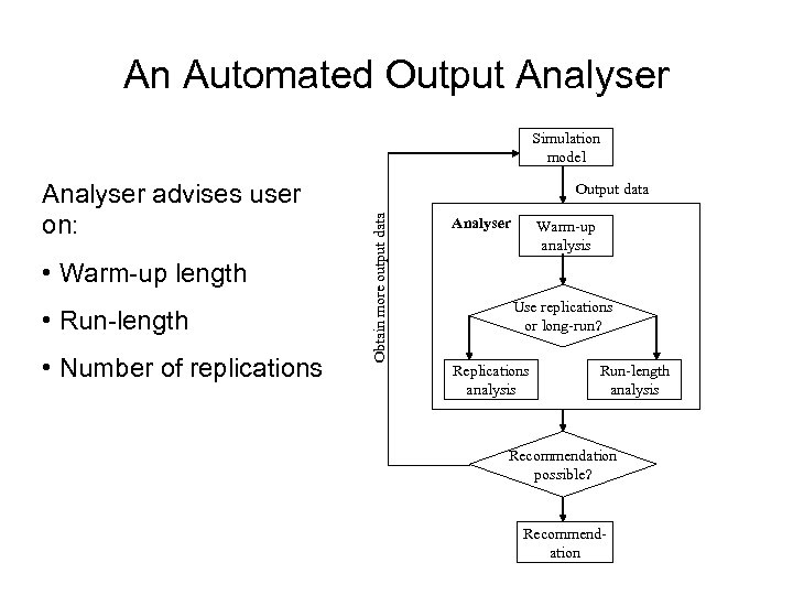An Automated Output Analyser Simulation model • Warm-up length • Run-length • Number of replications Output data Obtain more output data Analyser advises user on: Analyser Warm-up analysis Use replications or long-run? Replications analysis Run-length analysis Recommendation possible? Recommendation

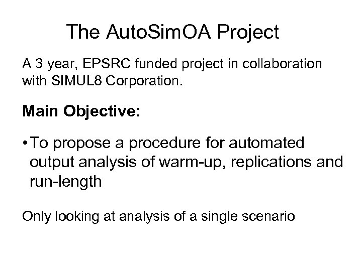The Auto. Sim. OA Project A 3 year, EPSRC funded project in collaboration with SIMUL 8 Corporation. Main Objective: • To propose a procedure for automated output analysis of warm-up, replications and run-length Only looking at analysis of a single scenario

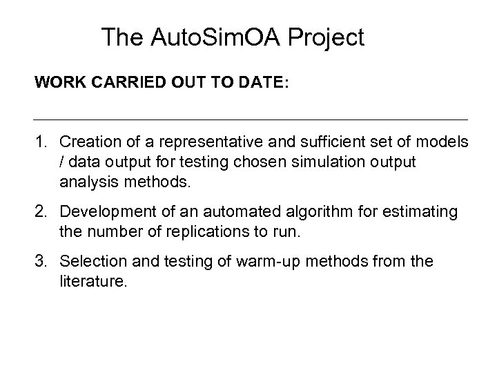The Auto. Sim. OA Project WORK CARRIED OUT TO DATE: 1. Creation of a representative and sufficient set of models / data output for testing chosen simulation output analysis methods. 2. Development of an automated algorithm for estimating the number of replications to run. 3. Selection and testing of warm-up methods from the literature.

Part 1. Creation of models and data sets

AIMS: Ø Provide a representative and sufficient set of models / data output for use in discrete event simulation research. Ø Use models / data sets to test the chosen simulation output analysis methods in the Auto. Sim. OA Project.

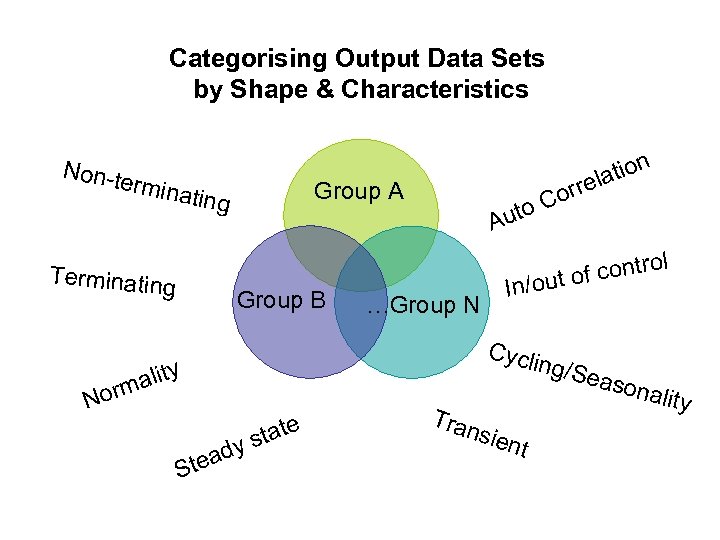Categorising Output Data Sets by Shape & Characteristics Non-t ermin Group A ating Terminating Group B Co to Au …Group N f contro /out o In Cycl ality orm N S tion a rrel d tea tate ys Tran sien t ing/S easo l nality

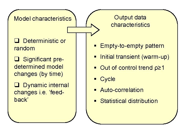Model characteristics q Deterministic or random q Significant predetermined model changes (by time) q Dynamic internal changes i. e. ‘feedback’ Output data characteristics § Empty-to-empty pattern § Initial transient (warm-up) § Out of control trend ρ≥ 1 § Cycle § Auto-correlation § Statistical distribution

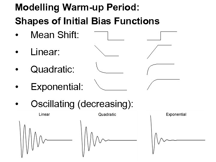Modelling Warm-up Period: Shapes of Initial Bias Functions • Mean Shift: • Linear: • Quadratic: • Exponential: • Oscillating (decreasing):

Artificial Data: Construct data which resembles real model output with known values for some specific attribute. Example: Known steady state mean and variance. Example data: AR(1) with N(0, 1) errors & linear initial bias. Real Models: Collect range of models created in “real circumstances”. Examples: • Swimming Pool complex: average number in system • Production Line Manufacturing Plant: through-put / hour • Fast Food Store: average queuing time

Part 2. WORK IN PROGRESS Automating estimation of warm-up length

The Initial Bias Problem • Model may not start in a “typical” state. • This may cause initial bias in the output. • Many methods proposed for dealing with initial bias: e. g. Initial steady state conditions; run model for ‘long’ time… • This project uses: Deletion of the initial transient data by specifying a warm-up period.

Question is: How do you estimate the length of the warm-up period required?

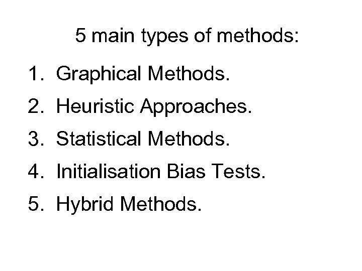5 main types of methods: 1. Graphical Methods. 2. Heuristic Approaches. 3. Statistical Methods. 4. Initialisation Bias Tests. 5. Hybrid Methods.

Literature search – 42 methods Summary of methods and literature references on project web site: http: //www. wbs. ac. uk/go/autosimoa Currently testing methods

Part 3. Automating analysis of number of replications

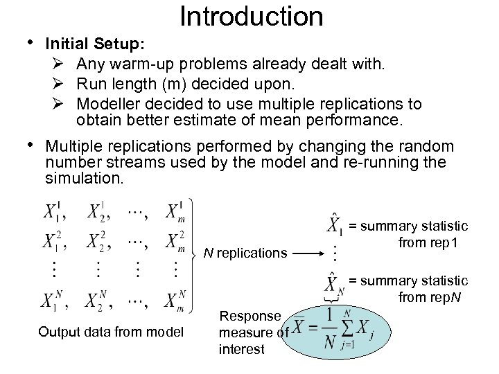• Initial Setup: Introduction Ø Any warm-up problems already dealt with. Ø Run length (m) decided upon. Ø Modeller decided to use multiple replications to obtain better estimate of mean performance. • Multiple replications performed by changing the random number streams used by the model and re-running the simulation. N replications = summary statistic from rep 1 = summary statistic from rep. N Output data from model Response measure of interest

QUESTION IS… How many replications are needed? • Limiting factors: computing time and expense. If performing N replications achieves a sufficient estimate of mean performance: > N replications: Unnecessary use of computer time and money. < N replications: Inaccurate results → incorrect decisions.

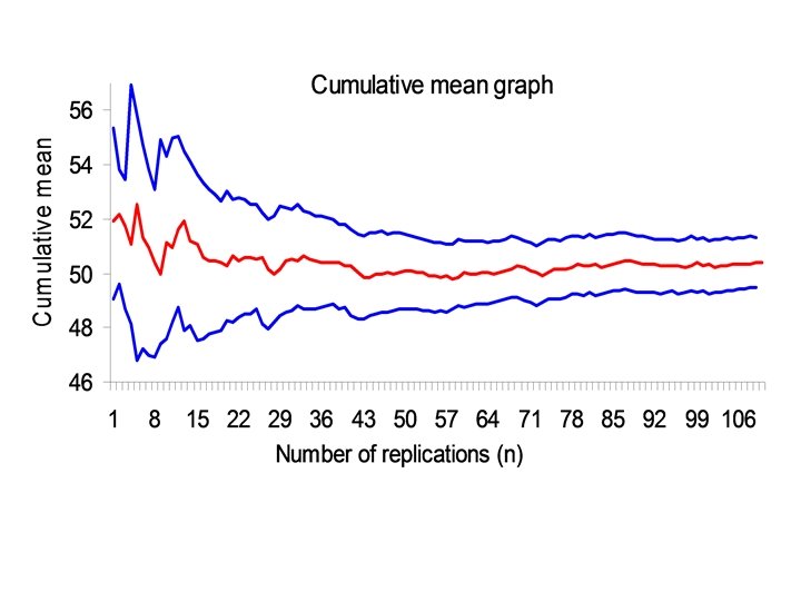
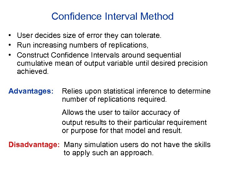Confidence Interval Method • User decides size of error they can tolerate. • Run increasing numbers of replications, • Construct Confidence Intervals around sequential cumulative mean of output variable until desired precision achieved. Advantages: Relies upon statistical inference to determine number of replications required. Allows the user to tailor accuracy of output results to their particular requirement or purpose for that model and result. Disadvantage: Many simulation users do not have the skills to apply such an approach.

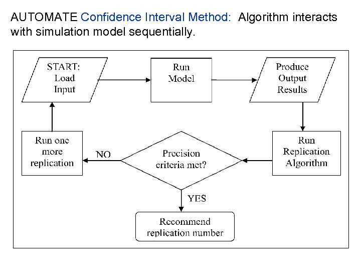AUTOMATE Confidence Interval Method: Algorithm interacts with simulation model sequentially.

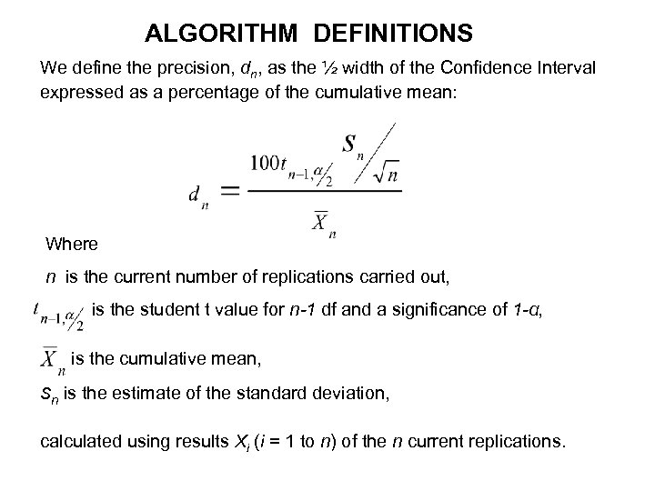ALGORITHM DEFINITIONS We define the precision, dn, as the ½ width of the Confidence Interval expressed as a percentage of the cumulative mean: Where n is the current number of replications carried out, is the student t value for n-1 df and a significance of 1 -α, is the cumulative mean, sn is the estimate of the standard deviation, calculated using results Xi (i = 1 to n) of the n current replications.

Stopping Criteria • Simplest method: Stop when dn 1 st found to be ≤ desired precision, drequired , and recommend that number of replications, Nsol, to the user. • Problem: Data series could prematurely converge, by chance, to incorrect estimate of the mean, with precision drequired , then diverge again. • ‘Look-ahead’ procedure: When dn 1 st found to be ≤ drequired, algorithm performs set number of extra replications, to check that precision remains ≤ drequired.

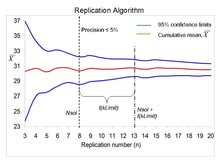Replication Algorithm 95% confidence limits Precision ≤ 5% Nsol f(k. Limit) Cumulative mean, Nsol + f(k. Limit)

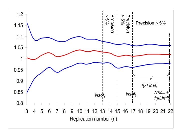Precision > 5% Precision ≤ 5% f(k. Limit) Nsol 1 Nsol 2 + f(k. Limit)

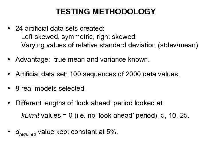TESTING METHODOLOGY • 24 artificial data sets created: Left skewed, symmetric, right skewed; Varying values of relative standard deviation (stdev/mean). • Advantage: true mean and variance known. • Artificial data set: 100 sequences of 2000 data values. • 8 real models selected. • Different lengths of ‘look ahead’ period looked at: k. Limit values = 0 (i. e. no ‘look ahead’ period), 5, 10, 25. • drequired value kept constant at 5%.

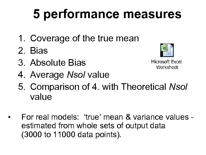5 performance measures 1. 2. 3. 4. 5. • Coverage of the true mean Bias Absolute Bias Average Nsol value Comparison of 4. with Theoretical Nsol value For real models: ‘true’ mean & variance values estimated from whole sets of output data (3000 to 11000 data points).

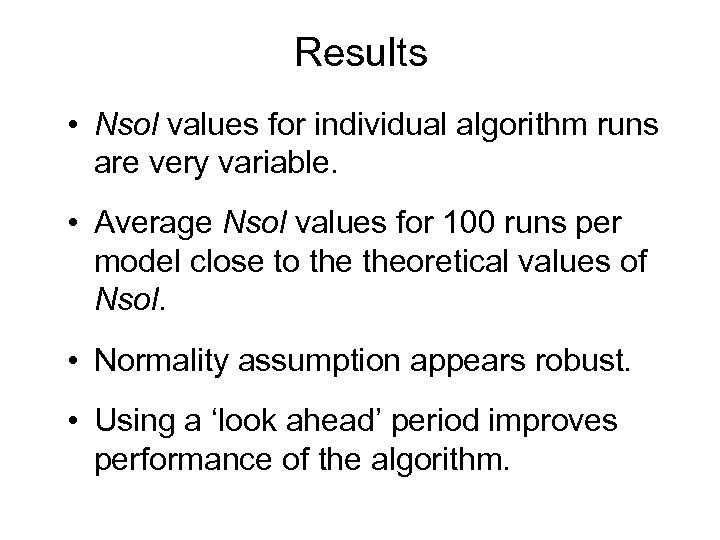Results • Nsol values for individual algorithm runs are very variable. • Average Nsol values for 100 runs per model close to theoretical values of Nsol. • Normality assumption appears robust. • Using a ‘look ahead’ period improves performance of the algorithm.

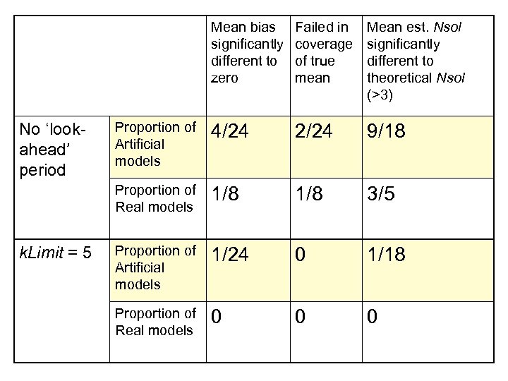Mean bias significantly different to zero k. Limit = 5 Mean est. Nsol significantly different to theoretical Nsol (>3) Proportion of Artificial models 4/24 2/24 9/18 Proportion of Real models No ‘lookahead’ period Failed in coverage of true mean 1/8 3/5 Proportion of Artificial models 1/24 0 1/18 Proportion of Real models 0 0 0

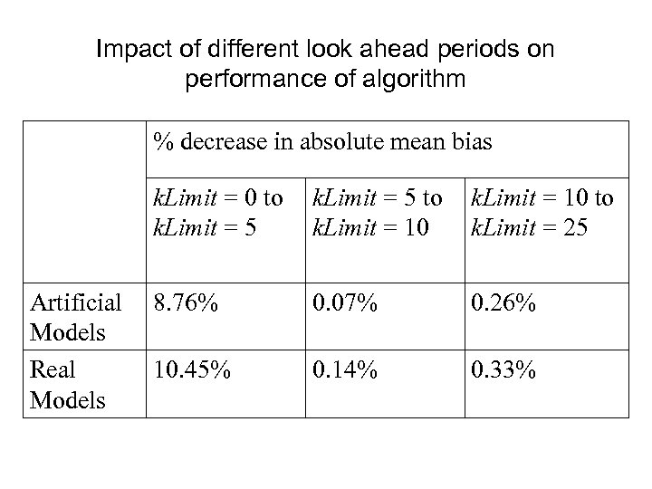Impact of different look ahead periods on performance of algorithm % decrease in absolute mean bias k. Limit = 0 to k. Limit = 5 Artificial Models Real Models k. Limit = 5 to k. Limit = 10 to k. Limit = 25 8. 76% 0. 07% 0. 26% 10. 45% 0. 14% 0. 33%

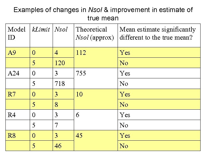Examples of changes in Nsol & improvement in estimate of true mean Model k. Limit Nsol ID Theoretical Mean estimate significantly Nsol (approx) different to the true mean? A 9 0 5 4 120 112 Yes No A 24 0 5 3 718 755 Yes No R 7 R 4 0 5 0 5 3 8 3 7 3 46 10 Yes No R 8 6 45

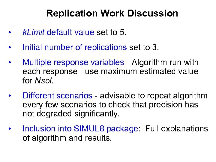Replication Work Discussion • k. Limit default value set to 5. • Initial number of replications set to 3. • Multiple response variables - Algorithm run with each response - use maximum estimated value for Nsol. • Different scenarios - advisable to repeat algorithm every few scenarios to check that precision has not degraded significantly. • Inclusion into SIMUL 8 package: Full explanations of algorithm and results.

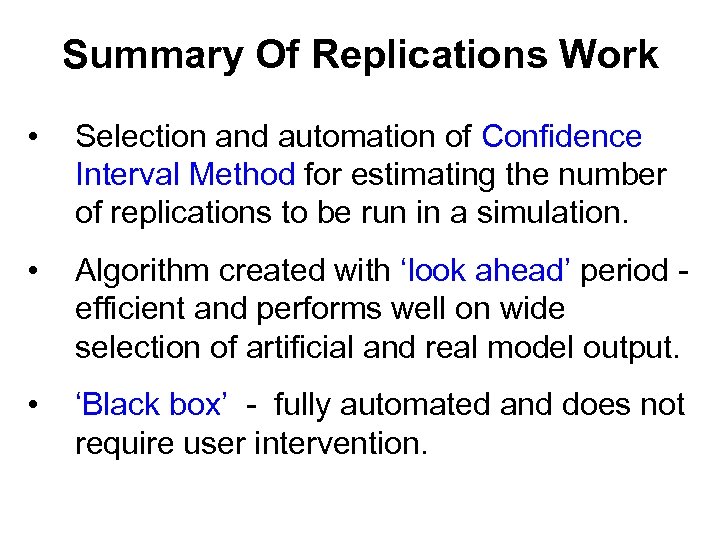Summary Of Replications Work • Selection and automation of Confidence Interval Method for estimating the number of replications to be run in a simulation. • Algorithm created with ‘look ahead’ period efficient and performs well on wide selection of artificial and real model output. • ‘Black box’ - fully automated and does not require user intervention.

PROJECT OVERVIEW • Created set of artificial and “real” model data including warm-up bias functions. • Created replication algorithm. Currently: • Testing warm-up methods.

ACKNOWLEDGMENTS This work is part of the Automating Simulation Output Analysis (Auto. Sim. OA) project that is funded by the UK (EPSRC) Engineering and Physical Sciences Research Council (EP/D 033640/1). The work is being carried out in collaboration with SIMUL 8 Corporation, who are also providing sponsorship for the project. Stewart Robinson, Katy Hoad, Ruth Davies SSIG Meeting, 24 th October 2007 http: //www. wbs. ac. uk/go/autosimoa