Automatic Transition Prediction in Unsteady Airfoil Flows Using

Automatic Transition Prediction in Unsteady Airfoil Flows Using an Unstructured CFD Code Andreas Krumbein, Normann Krimmelbein, Cornelia Seyfert German Aerospace Center Institute of Aerodynamics and Flow Technology C²A²S²E Center for Computer Applications in Aero. Space Science and Engineering 29 th AIAA Applied Aerodynamics Conference, Honolulu, Hawaii, Slide 1 Andreas Krumbein > 28 June 2011

Overview Introduction Transition Prediction Coupling Structure Extension of the e. N method for unsteady base flows Test Cases & Computational Results Conclusion & Outlook 2 Andreas Krumbein > 28 June 2011

Introduction Transition Prediction in RANS-based CFD of External Flows Current status of transition prediction in RANS solvers have become a standard approach for the design and the aerodynamic analysis of aerodynamic configurations. Requirement from Aircraft Industry and Research for a long time: RANS solver with integrated general transition prediction functionality Automatic: no intervention of the user Autonomous: as little additional information as possible Major aims: Reduction of modeling based uncertainties Improvement of simulation accuracy Accuracy of results from fully turbulent computations or from computations with prescribed transition often not satisfactory Exploitation of the full potential of advanced turbulence models Most important, at present, improved simulation of the interaction between transition locations and separation, especially for high-lift configurations. 3 Andreas Krumbein > 28 June 2011

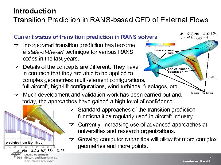Introduction Transition Prediction in RANS-based CFD of External Flows Current status of transition prediction in RANS solvers Incorporated transition prediction has become a state-of-the-art technique for various RANS codes in the last years. M = 0. 2, Re = 2. 3 x 106, a = -4. 0°, i. HTP = 4° inviscid stream lines Details of the concepts are different. They have line of laminar separation in common that they are able to be applied to complex geometries: multi-element configurations, full aircraft, high-lift configurations, wind turbines, fuselages, etc. transition lines Much development and validation work has been carried out and, today, the approaches have gained a high level of confidence. Standard approaches of the transition prediction functionalities regularly used in aircraft industry. Currently, increasing use of advanced approaches at universities and research organizations. Growing computer capacities will allow for more complex predicted transition lines geometries and more points. Re = 3. 5 x 106, Ma = 0. 17 4 Andreas Krumbein > 28 June 2011

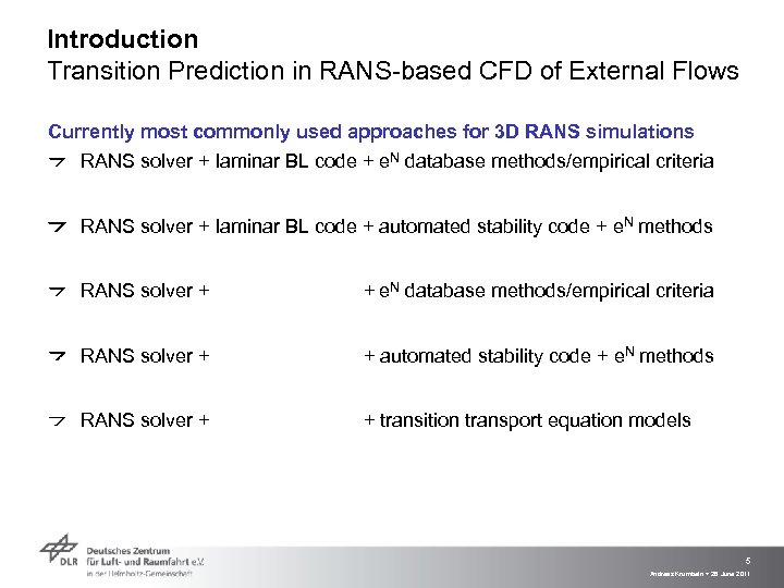Introduction Transition Prediction in RANS-based CFD of External Flows Currently most commonly used approaches for 3 D RANS simulations RANS solver + laminar BL code + e. N database methods/empirical criteria RANS solver + laminar BL code + automated stability code + e. N methods RANS solver + + e. N database methods/empirical criteria RANS solver + + automated stability code + e. N methods RANS solver + + transition transport equation models 5 Andreas Krumbein > 28 June 2011

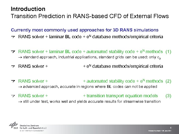Introduction Transition Prediction in RANS-based CFD of External Flows Currently most commonly used approaches for 3 D RANS simulations RANS solver + laminar BL code + e. N database methods/empirical criteria RANS solver + laminar BL code + automated stability code + e. N methods (1) standard approach, industrial applications, standard grids can be used: only cp RANS solver + + e. N database methods/empirical criteria RANS solver + + automated stability code + e. N methods (2) advanced approach, accurate in regions where BL codes can not be applied RANS solver + + transition transport equation models (3) still under test, works well and yields accurate results for streamwise transition 6 Andreas Krumbein > 28 June 2011

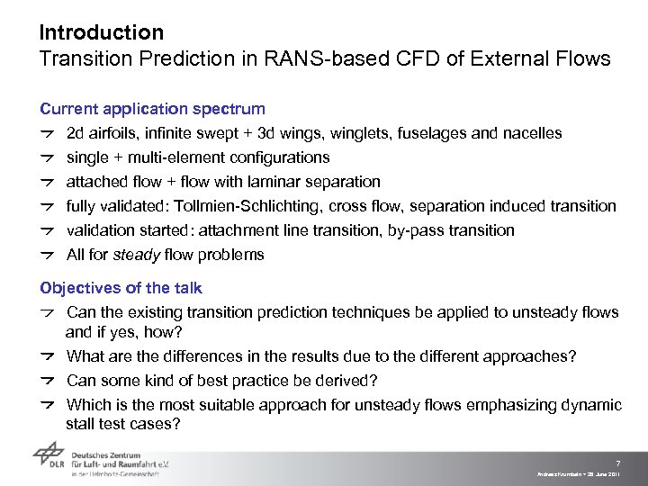Introduction Transition Prediction in RANS-based CFD of External Flows Current application spectrum 2 d airfoils, infinite swept + 3 d wings, winglets, fuselages and nacelles single + multi-element configurations attached flow + flow with laminar separation fully validated: Tollmien-Schlichting, cross flow, separation induced transition validation started: attachment line transition, by-pass transition All for steady flow problems Objectives of the talk Can the existing transition prediction techniques be applied to unsteady flows and if yes, how? What are the differences in the results due to the different approaches? Can some kind of best practice be derived? Which is the most suitable approach for unsteady flows emphasizing dynamic stall test cases? 7 Andreas Krumbein > 28 June 2011

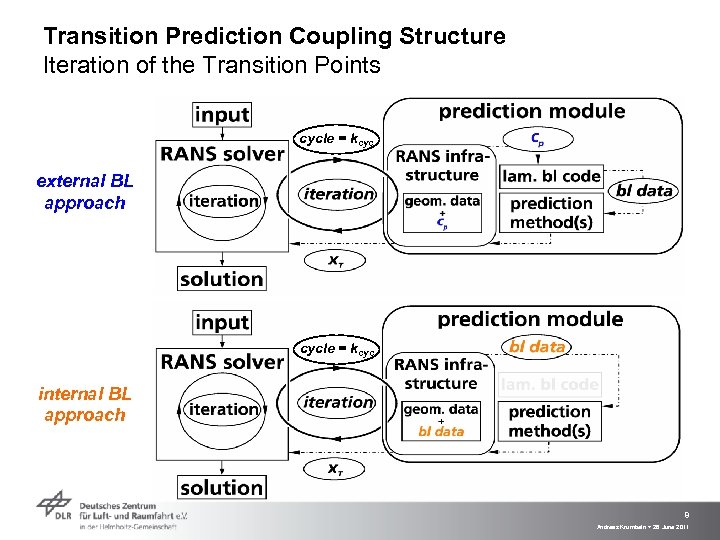Transition Prediction Coupling Structure Iteration of the Transition Points cycle = kcyc external BL approach cycle = kcyc internal BL approach 8 Andreas Krumbein > 28 June 2011

Transition Prediction Coupling Structure Transition Prediction Module Treatment of separation induced transition external BL approach Yields very accurate laminar BL profiles using grids with standard resolution. BL code stops at the point of laminar separation. The laminar separation point approximates the transition point if transition is located downstream of the separation point. internal BL approach Needs very fine grid resolution in wall normal direction for sufficient accuracy of laminar BL profiles including the 1 st and 2 nd derivatives which are input for the stability code, ≈ 40 points in prismatic layer of a hybrid grid for streamwise instabilities. Stability analysis can be carried out inside the separation bubble. Sufficiently high resolution of the bubble must be ensured also in streamwise direction, factor 2÷ 2. 5 compared to normal resolution (≈ 256 points airfoil contour). 9 Andreas Krumbein > 28 June 2011

Transition Prediction Coupling Structure Unstructured RANS Solver TAU 3 D RANS, compressible, steady/unsteady Hybrid unstructured grids: hexahedra, tetrahedra, pyramids, prisms Finite volume formulation Vertex-centered spatial scheme (edge-based dual-cell approach) 2 nd order central scheme, scalar or matrix artificial dissipation Pseudo-time integration: explicit Runge-Kutta or implicit approximate factorization scheme (LU-SGS), multi-grid acceleration, local time stepping, explicit residual smoothing, low Mach number preconditioning Physical time integration: dual time stepping using pseudo-time integration for the inner iterations Turbulence models: 1 - and 2 -equation eddy viscosity models (SA type, k-w type) differential RSM DES 10 Andreas Krumbein > 28 June 2011

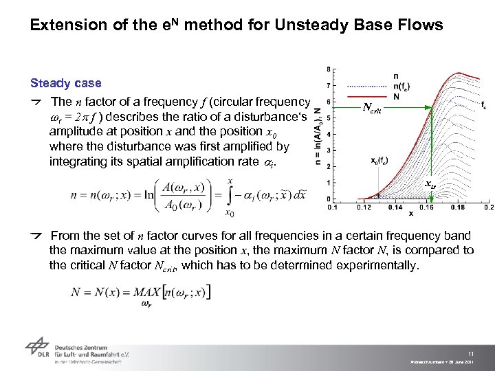Extension of the e. N method for Unsteady Base Flows Steady case The n factor of a frequency f (circular frequency wr = 2 p f ) describes the ratio of a disturbance‘s amplitude at position x and the position x 0 where the disturbance was first amplified by integrating its spatial amplification rate ai. Ncrit xtr From the set of n factor curves for all frequencies in a certain frequency band the maximum value at the position x, the maximum N factor N, is compared to the critical N factor Ncrit, which has to be determined experimentally. 11 Andreas Krumbein > 28 June 2011

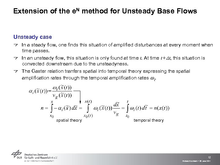Extension of the e. N method for Unsteady Base Flows Unsteady case In a steady flow, one finds this situation of amplified disturbances at every moment when time passes. In an unsteady flow, this situation is only found at time t. At time t +Dt, this situation is convected downstream due to the unsteadyness. The Gaster relation tranfers spatial into temporal theory expressing the spatial amplification rates through the temporal amplification rates wi. spatial theory temporal theory 12 Andreas Krumbein > 28 June 2011

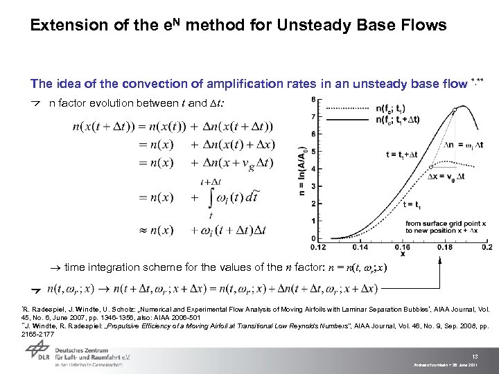Extension of the e. N method for Unsteady Base Flows The idea of the convection of amplification rates in an unsteady base flow n factor evolution between t and Dt: *, ** time integration scheme for the values of the n factor: n = n(t, wr; x) *R. Radespiel, J. Windte, U. Scholz: „Numerical and Experimental Flow Analysis of Moving Airfoils with Laminar Separation Bubbles‘, AIAA Journal, Vol. 45, No. 6, June 2007, pp. 1346 -1356, also: AIAA 2006 -501 **J. Windte, R. Radespiel: „Propulsive Efficiency of a Moving Airfoil at Transitional Low Reynolds Numbers“, AIAA Journal, Vol. 46, No. 9, Sep. 2008, pp. 2165 -2177 13 Andreas Krumbein > 28 June 2011

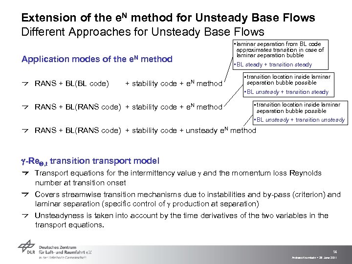Extension of the e. N method for Unsteady Base Flows Different Approaches for Unsteady Base Flows Application modes of the e. N method RANS + BL(BL code) + stability code + e. N method • laminar separation from BL code approximates transition in case of laminar separation bubble • BL steady + transition steady • transition location inside laminar separation bubble possible • BL unsteady + transition steady RANS + BL(RANS code) + stability code + e. N method • transition location inside laminar separation bubble possible • BL unsteady + transition unsteady RANS + BL(RANS code) + stability code + unsteady e. N method g-Re. Q, t transition transport model Transport equations for the intermittency value g and the momentum loss Reynolds number at transition onset Covers streamwise transition mechanisms due to instabilities and by-pass (criterion) and laminar separation (specific control of g production at separation) Unsteadyness is taken into account by the time derivatives of the two variables in the transport equations. 14 Andreas Krumbein > 28 June 2011

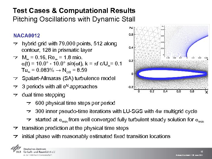Test Cases & Computational Results Pitching Oscillations with Dynamic Stall NACA 0012 hybrid grid with 79, 000 points, 512 along contour, 128 in prismatic layer M = 0. 16, Re = 1. 8 mio. a(t) = 10. 0° - 10. 0° sin(wt), k = pf c/U = 0. 1 Tu∞ = 0. 083% → Ncrit = 8. 59 Spalart-Allmaras (SA) turbulence model 3 periods with all e. N approaches dual time stepping 600 physical time steps period 300 inner pseudo-time iterations with LU-SGS with 4 w multigrid cycle started at amin from well converged fully turbulent steady solution for amin transition prediction at the physical time steps initial phase with reasonably estimated fixed transition locations 15 Andreas Krumbein > 28 June 2011

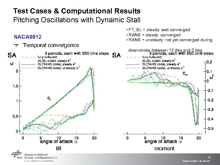Test Cases & Computational Results Pitching Oscillations with Dynamic Stall NACA 0012 Temporal convergence lift ▪ FT, BL + steady: well converged ▪ RANS + steady: converged ▪ RANS + unsteady: not yet converged during downstroke between 13 deg and 0 deg moment 16 Andreas Krumbein > 28 June 2011

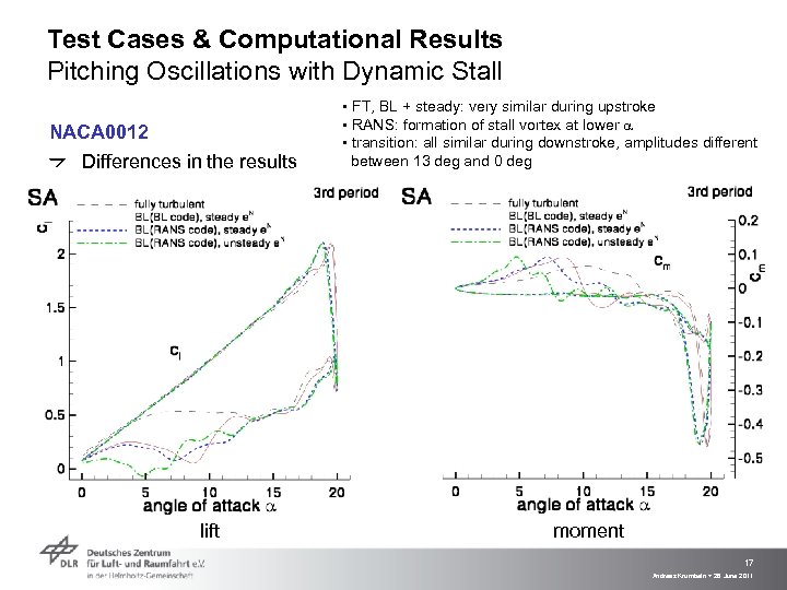Test Cases & Computational Results Pitching Oscillations with Dynamic Stall NACA 0012 Differences in the results lift ▪ FT, BL + steady: very similar during upstroke ▪ RANS: formation of stall vortex at lower a ▪ transition: all similar during downstroke, amplitudes different between 13 deg and 0 deg moment 17 Andreas Krumbein > 28 June 2011

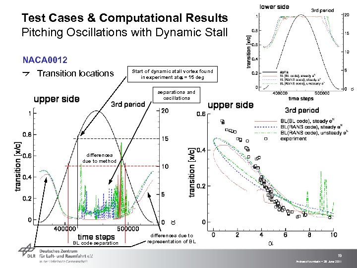Test Cases & Computational Results Pitching Oscillations with Dynamic Stall NACA 0012 Transition locations Start of dynamic stall vortex found in experiment at = 15 deg separations and oscillations differences due to method BL code separation differences due to representation of BL 18 Andreas Krumbein > 28 June 2011

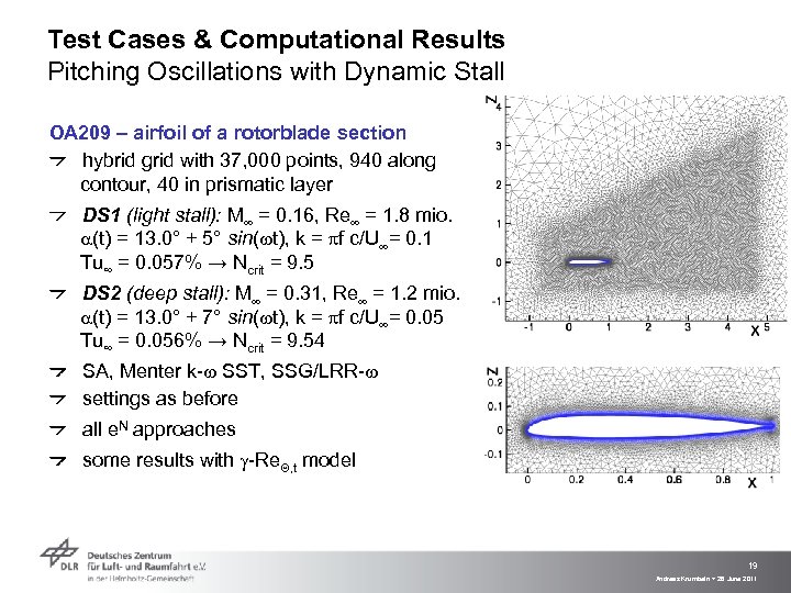Test Cases & Computational Results Pitching Oscillations with Dynamic Stall OA 209 – airfoil of a rotorblade section hybrid grid with 37, 000 points, 940 along contour, 40 in prismatic layer DS 1 (light stall): M = 0. 16, Re = 1. 8 mio. a(t) = 13. 0° + 5° sin(wt), k = pf c/U = 0. 1 Tu∞ = 0. 057% → Ncrit = 9. 5 DS 2 (deep stall): M = 0. 31, Re = 1. 2 mio. a(t) = 13. 0° + 7° sin(wt), k = pf c/U = 0. 05 Tu∞ = 0. 056% → Ncrit = 9. 54 SA, Menter k-w SST, SSG/LRR-w settings as before all e. N approaches some results with g-Re. Q, t model 19 Andreas Krumbein > 28 June 2011

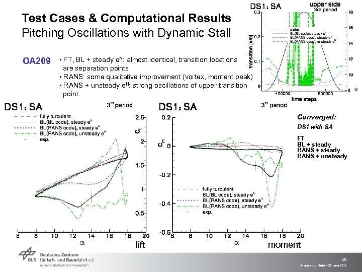Test Cases & Computational Results Pitching Oscillations with Dynamic Stall OA 209 ▪ FT, BL + steady e. N: almost identical, transition locations are separation points ▪ RANS: some qualitative improvement (vortex, moment peak) ▪ RANS + unsteady e. N: strong oscillations of upper transition point Converged: DS 1 with SA FT BL + steady RANS + unsteady lift moment 20 Andreas Krumbein > 28 June 2011

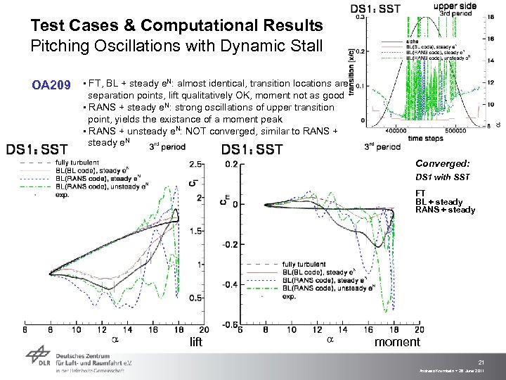Test Cases & Computational Results Pitching Oscillations with Dynamic Stall OA 209 ▪ FT, BL + steady e. N: almost identical, transition locations are separation points, lift qualitatively OK, moment not as good ▪ RANS + steady e. N: strong oscillations of upper transition point, yields the existance of a moment peak ▪ RANS + unsteady e. N: NOT converged, similar to RANS + steady e. N Converged: DS 1 with SST FT BL + steady RANS + steady lift moment 21 Andreas Krumbein > 28 June 2011

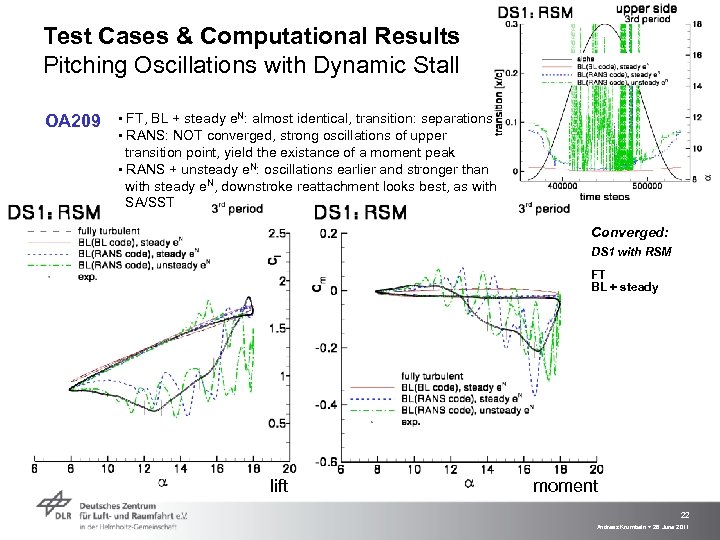Test Cases & Computational Results Pitching Oscillations with Dynamic Stall OA 209 ▪ FT, BL + steady e. N: almost identical, transition: separations ▪ RANS: NOT converged, strong oscillations of upper transition point, yield the existance of a moment peak ▪ RANS + unsteady e. N: oscillations earlier and stronger than with steady e. N, downstroke reattachment looks best, as with SA/SST Converged: DS 1 with RSM FT BL + steady lift moment 22 Andreas Krumbein > 28 June 2011

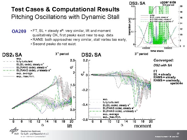Test Cases & Computational Results Pitching Oscillations with Dynamic Stall OA 209 ▪ FT, BL + steady e. N: very similar, lift and moment qualitatively OK, first peaks exist near to exp. data ▪ RANS: both approaches very similar, stall vortex too early, ▪ Second peaks do not exist. Converged: DS 2 with SA FT BL + steady RANS + unsteady, upstroke lift moment 23 Andreas Krumbein > 28 June 2011

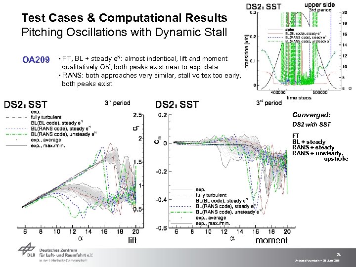Test Cases & Computational Results Pitching Oscillations with Dynamic Stall OA 209 ▪ FT, BL + steady e. N: almost indentical, lift and moment qualitatively OK, both peaks exist near to exp. data ▪ RANS: both approaches very similar, stall vortex too early, both peaks exist Converged: DS 2 with SST FT BL + steady RANS + unsteady, upstroke lift moment 24 Andreas Krumbein > 28 June 2011

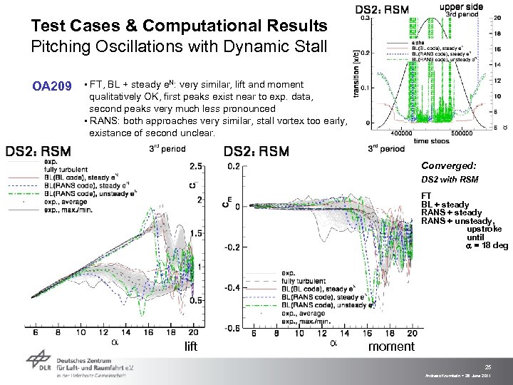Test Cases & Computational Results Pitching Oscillations with Dynamic Stall OA 209 ▪ FT, BL + steady e. N: very similar, lift and moment qualitatively OK, first peaks exist near to exp. data, second peaks very much less pronounced ▪ RANS: both approaches very similar, stall vortex too early, existance of second unclear. Converged: DS 2 with RSM FT BL + steady RANS + unsteady, upstroke until = 18 deg lift moment 25 Andreas Krumbein > 28 June 2011

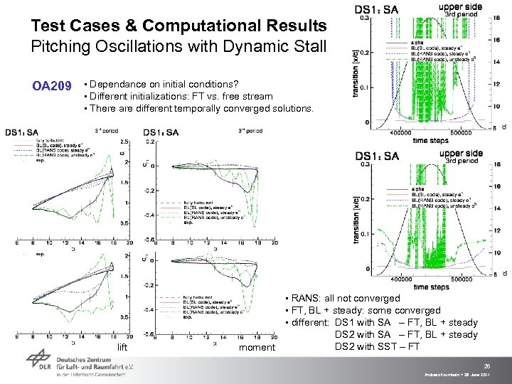Test Cases & Computational Results Pitching Oscillations with Dynamic Stall OA 209 ▪ Dependance on initial conditions? ▪ Different initializations: FT vs. free stream ▪ There are different temporally converged solutions. lift moment ▪ RANS: all not converged ▪ FT, BL + steady: some converged ▪ different: DS 1 with SA – FT, BL + steady DS 2 with SST – FT 26 Andreas Krumbein > 28 June 2011

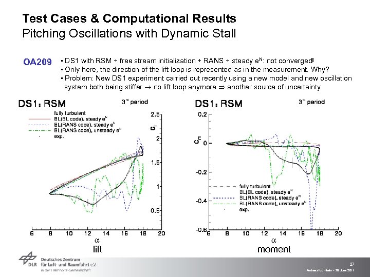Test Cases & Computational Results Pitching Oscillations with Dynamic Stall OA 209 ▪ DS 1 with RSM + free stream initialization + RANS + steady e. N: not converged! ▪ Only here, the direction of the lift loop is represented as in the measurement. Why? ▪ Problem: New DS 1 experiment carried out recently using a new model and new oscillation system both being stiffer no lift loop anymore another source of uncertainty lift moment 27 Andreas Krumbein > 28 June 2011

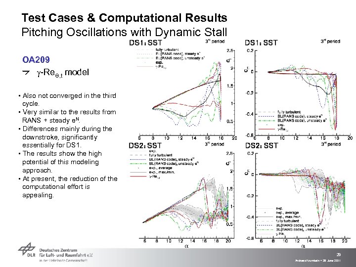Test Cases & Computational Results Pitching Oscillations with Dynamic Stall OA 209 g-Re. Q, t model ▪ Also not converged in the third cycle. ▪ Very similar to the results from RANS + steady e. N. ▪ Differences mainly during the downstroke, significantly essentially for DS 1. ▪ The results show the high potential of this modeling approach. ▪ At present, the reduction of the computational effort is appealing. 28 Andreas Krumbein > 28 June 2011

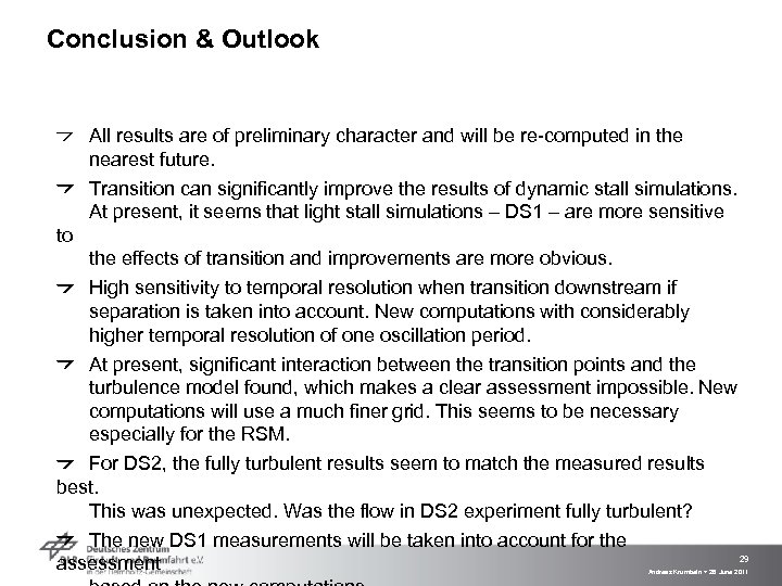Conclusion & Outlook All results are of preliminary character and will be re-computed in the nearest future. Transition can significantly improve the results of dynamic stall simulations. At present, it seems that light stall simulations – DS 1 – are more sensitive to the effects of transition and improvements are more obvious. High sensitivity to temporal resolution when transition downstream if separation is taken into account. New computations with considerably higher temporal resolution of one oscillation period. At present, significant interaction between the transition points and the turbulence model found, which makes a clear assessment impossible. New computations will use a much finer grid. This seems to be necessary especially for the RSM. For DS 2, the fully turbulent results seem to match the measured results best. This was unexpected. Was the flow in DS 2 experiment fully turbulent? The new DS 1 measurements will be taken into account for the 29 assessment Andreas Krumbein > 28 June 2011

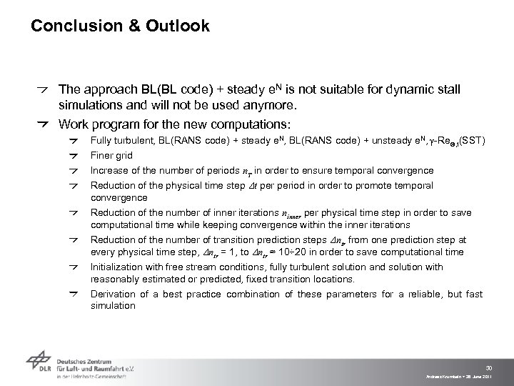Conclusion & Outlook The approach BL(BL code) + steady e. N is not suitable for dynamic stall simulations and will not be used anymore. Work program for the new computations: Fully turbulent, BL(RANS code) + steady e. N, BL(RANS code) + unsteady e. N, g-Re. Q, t(SST) Finer grid Increase of the number of periods n. T in order to ensure temporal convergence Reduction of the physical time step Dt period in order to promote temporal convergence Reduction of the number of inner iterations ninner physical time step in order to save computational time while keeping convergence within the inner iterations Reduction of the number of transition prediction steps Dntr from one prediction step at every physical time step, Dntr = 1, to Dntr ≈ 10÷ 20 in order to save computational time Initialization with free stream conditions, fully turbulent solution and solution with reasonably estimated or predicted, fixed transition locations. Derivation of a best practice combination of these parameters for a reliable, but fast simulation 30 Andreas Krumbein > 28 June 2011