Automated Construction of Environment Models by a Mobile

Automated Construction of Environment Models by a Mobile Robot Thesis Proposal Paul Blaer January 5, 2005

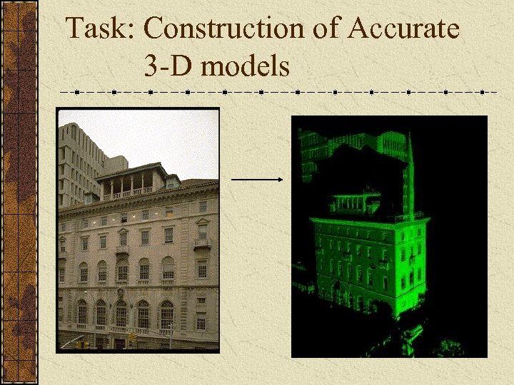
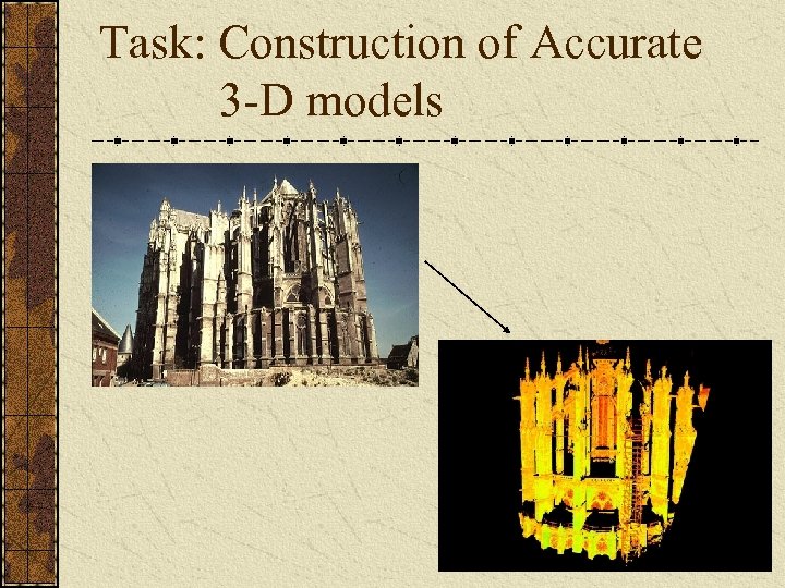
Task: Construction of Accurate 3 -D models

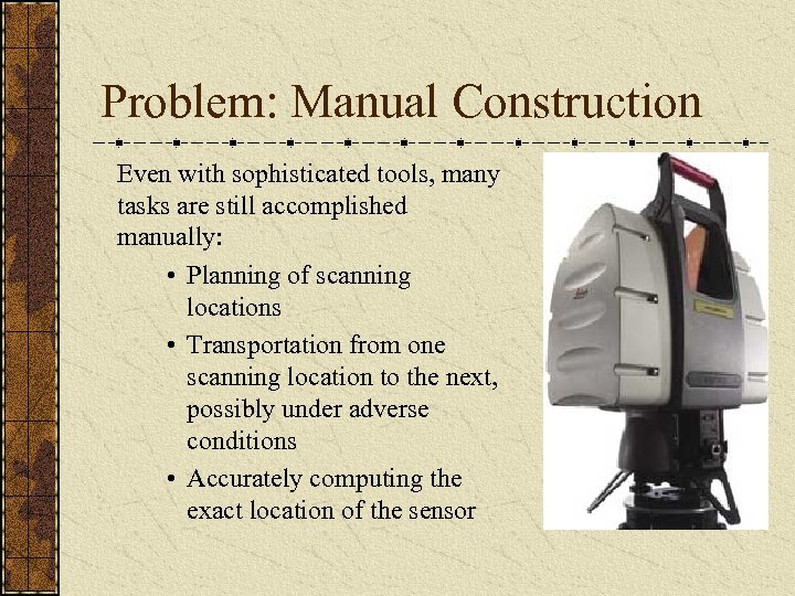
Problem: Manual Construction Even with sophisticated tools, many tasks are still accomplished manually: • Planning of scanning locations • Transportation from one scanning location to the next, possibly under adverse conditions • Accurately computing the exact location of the sensor

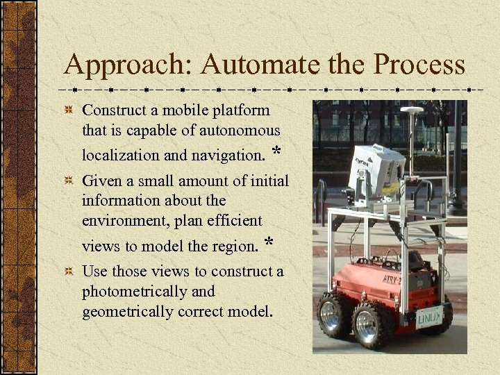
Approach: Automate the Process Construct a mobile platform that is capable of autonomous localization and navigation. * Given a small amount of initial information about the environment, plan efficient views to model the region. * Use those views to construct a photometrically and geometrically correct model.

Proposed Contributions: An improved 2 -D view planning algorithm used for bootstrapping the construction of a complete scene model A new 3 -D voxel-based next-best-view algorithm A topological localization algorithm combining omnidirectional vision and wireless access point signals. Voronoi diagram-based path planner for navigation. A model construction system that fuses the view planning algorithms with the robot’s navigation and control systems.

Large Scale 3 -D Modeling Literature: 1. 3 D City Model Construction at Berkeley – Frueh, et al, 2004, 2002 2. Outdoor Map Building at University of Tsukuba – Ohno, et al 2004 3. MIT City Scanning Project – Teller, 1997 4. Klein and Sequeira, 2004, 2000 5. Nuchter, et al, 2003

View Planning Literature: 1. Model Based Methods • Cowan and Kovesi, 1988 • Tarabanis and Tsai, 1992 • Tarabanis, et al, 1995 • Tarbox and Gottschlich, 1995 • Scott, Roth and Rivest, 2001 3. Art Gallery Methods • Xie, et al, 1986 • Gonzalez-Banos, et al, 1997 • Danner and Kavraki, 2000 4. View Planning for Mobile Robots • Gonzalez-Banos, et al, 2000 • Grabowski, et al, 2003 • Nuchter, et al, 2003 2. Non-Model Based Methods • Volumetric Methods – Connolly, 1985 – Banta et al, 1995 – Massios and Fisher, 1998 – Papadopoulos-Organos, 1997 – Soucey, et al, 1998 • Surface-Based Methods – Maver and Bajcsy, 1993 – Yuan, 1995 – Zha, et al, 1997 – Pito, 1999 – Reed and Allen, 2000 – Klein and Sequeira, 2000 • Whaite and Ferrie, 1997

Overview of Our System Platform Steps in Our Method Initial Modeling Stage Planning the Robot’s Paths Localization and Navigation Acquiring the Scan Final Modeling Stage Testbeds

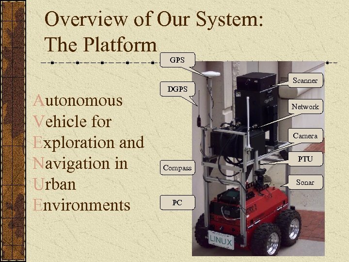
Overview of Our System: The Platform GPS Scanner Autonomous Vehicle for Exploration and Navigation in Urban Environments DGPS Network Camera PTU Compass Sonar PC

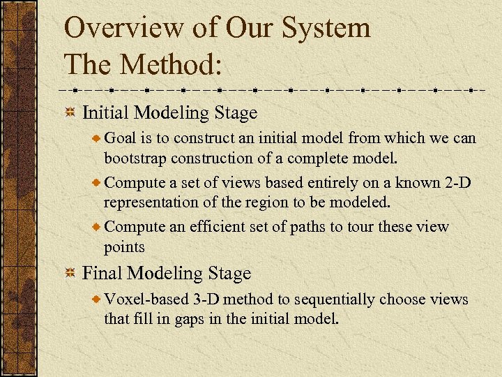
Overview of Our System The Method: Initial Modeling Stage Goal is to construct an initial model from which we can bootstrap construction of a complete model. Compute a set of views based entirely on a known 2 -D representation of the region to be modeled. Compute an efficient set of paths to tour these view points Final Modeling Stage Voxel-based 3 -D method to sequentially choose views that fill in gaps in the initial model.

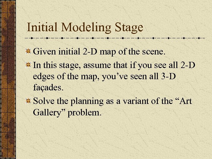
Initial Modeling Stage Given initial 2 -D map of the scene. In this stage, assume that if you see all 2 -D edges of the map, you’ve seen all 3 -D façades. Solve the planning as a variant of the “Art Gallery” problem.

Initial Modeling Stage Problems with the “Art Gallery” approach: Traditional geometric approaches assume that the guards can see 360 o around with unlimited range, ignoring any constraints of the scanner. A view of the 2 -D footprint of an obstacle does not necessarily mean that we have seen the entire façade. There may be interesting 3 -D structure above.

Initial Modeling Stage A randomized algorithm for the 2 -D problem: First choose a random set of potential views in the free space

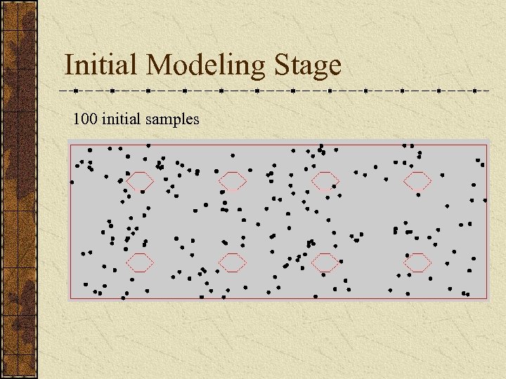
Initial Modeling Stage 100 initial samples

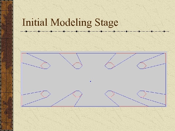
Initial Modeling Stage A randomized algorithm for the 2 -D problem: First choose a random set of potential views in the free space Compute the visibility of each potential view

Initial Modeling Stage

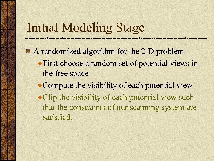
Initial Modeling Stage A randomized algorithm for the 2 -D problem: First choose a random set of potential views in the free space Compute the visibility of each potential view Clip the visibility of each potential view such that the constraints of our scanning system are satisfied.

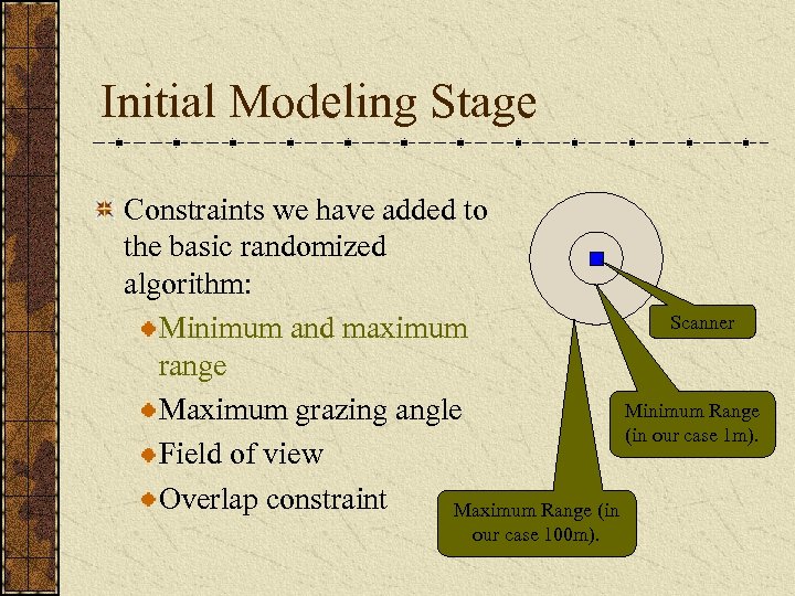
Initial Modeling Stage Constraints we have added to the basic randomized algorithm: Scanner Minimum and maximum range Minimum Range Maximum grazing angle (in our case 1 m). Field of view Overlap constraint Maximum Range (in our case 100 m).

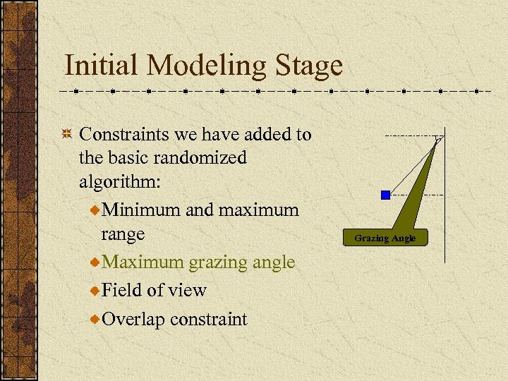
Initial Modeling Stage Constraints we have added to the basic randomized algorithm: Minimum and maximum range Maximum grazing angle Field of view Overlap constraint Grazing Angle

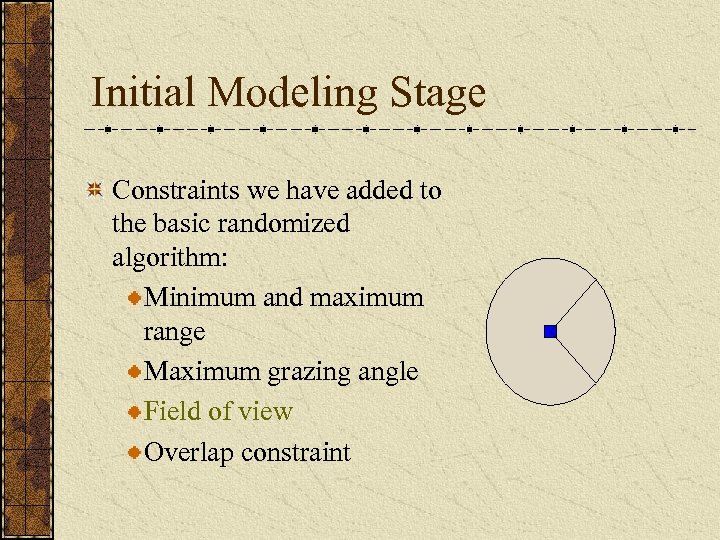
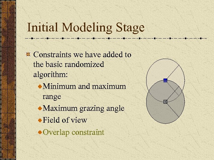
Initial Modeling Stage Constraints we have added to the basic randomized algorithm: Minimum and maximum range Maximum grazing angle Field of view Overlap constraint

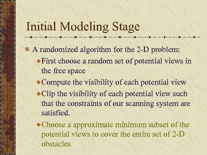
Initial Modeling Stage A randomized algorithm for the 2 -D problem: First choose a random set of potential views in the free space Compute the visibility of each potential view Clip the visibility of each potential view such that the constraints of our scanning system are satisfied. Choose a approximate minimum subset of the potential views to cover the entire set of 2 -D obstacles

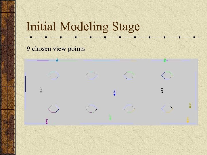
Initial Modeling Stage 9 chosen view points

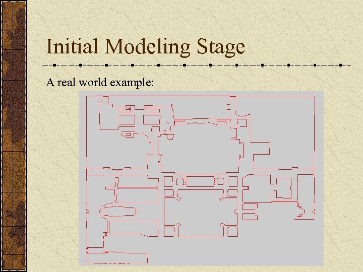
Initial Modeling Stage A real world example:

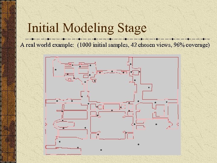
Initial Modeling Stage A real world example: (1000 initial samples, 42 chosen views, 96% coverage)

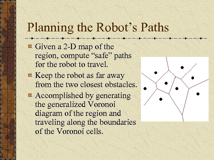
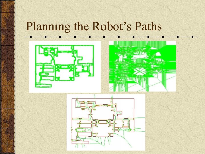
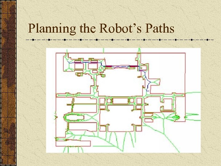
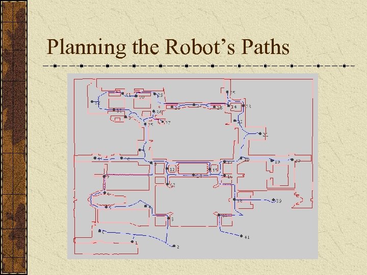
Planning the Robot’s Paths Given a 2 -D map of the region, compute “safe” paths for the robot to travel. Keep the robot as far away from the two closest obstacles. Accomplished by generating the generalized Voronoi diagram of the region and traveling along the boundaries of the Voronoi cells.

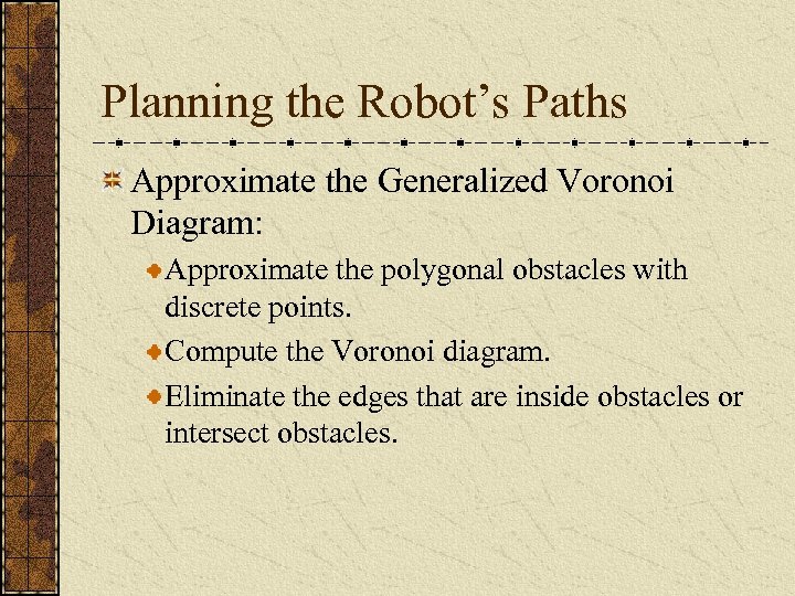
Planning the Robot’s Paths Approximate the Generalized Voronoi Diagram: Approximate the polygonal obstacles with discrete points. Compute the Voronoi diagram. Eliminate the edges that are inside obstacles or intersect obstacles.

Planning the Robot’s Paths

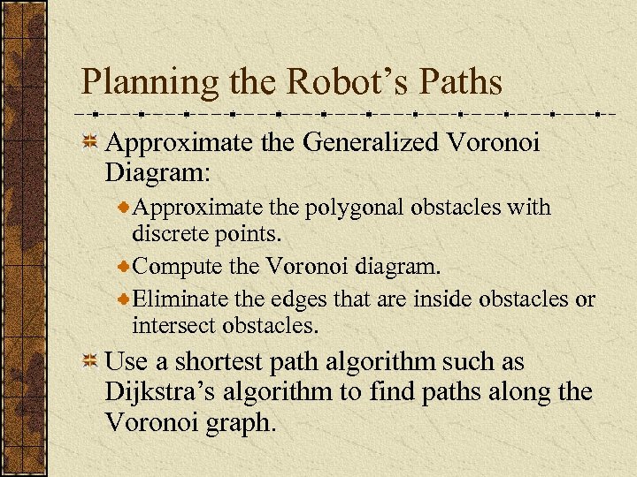
Planning the Robot’s Paths Approximate the Generalized Voronoi Diagram: Approximate the polygonal obstacles with discrete points. Compute the Voronoi diagram. Eliminate the edges that are inside obstacles or intersect obstacles. Use a shortest path algorithm such as Dijkstra’s algorithm to find paths along the Voronoi graph.

Planning the Robot’s Paths

Planning the Robot’s Paths Need to generate a tour for the robot to visit all the initially selected view points. This can be treated as a “Traveling Salesman Problem” and solved with any number of approximations. To generate edge weights, we first compute our “safe” Voronoi paths between all viewpoints. We use the lengths of those paths as the edge weights for our graph.

Planning the Robot’s Paths

Localization and Navigation Existing system uses a combination of: GPS Odometry Attitude Sensor Fine grained visual localization (Georgiev and Allen, 2004) Problems: GPS can fail in urban canyons Odometry is unreliable because of slipping and cumulative error Fine grained visual localization system needs an existing position estimate

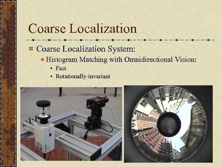
Coarse Localization System: Histogram Matching with Omnidirectional Vision: • Fast • Rotationally-invariant

Coarse Localization System: Histogram Matching with Omnidirectional Vision: • Fast • Rotationally-invariant Wireless signal strength of Access Points Use existing wireless infrastructure to resolve ambiguities in location. Look at the signal strengths to all visible base stations at a given location and compare against database.

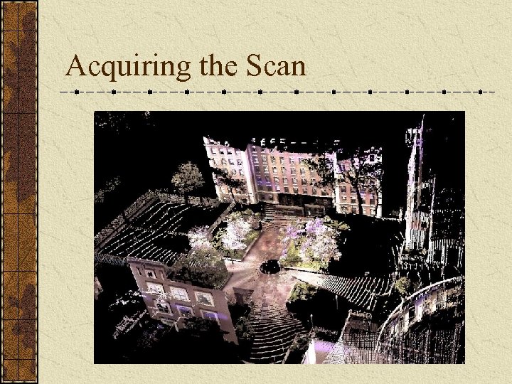
Acquiring the Scan

Final Modeling Stage The initial modeling stage will result in an incomplete model: Undetectable 3 -D occlusions Previously unknown obstacles Temporary obstacles Need a second modeling stage to fill in the holes.

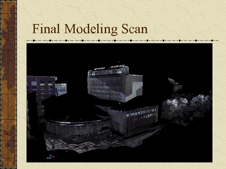
Final Modeling Scan

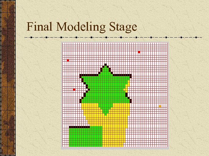
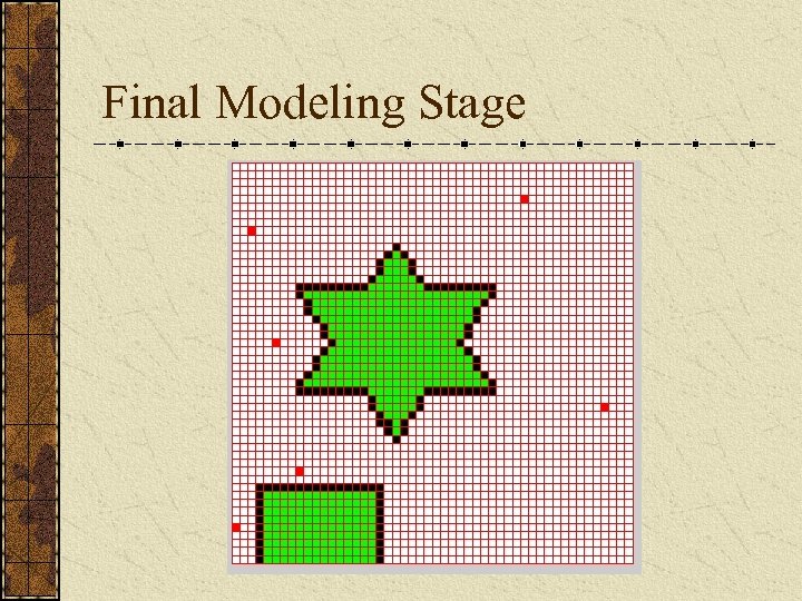
Final Modeling Stage We store the world as a voxel grid. For view planning of large scenes the voxels do not need to be small. Initial voxel grid is populated with the scans from the first stage. • If a voxel has a data point in it, it is marked as seenoccupied. • Unoccupied voxels along the straight line path from that point back to its scanning location that are marked as seen-empty. • All other voxels are marked as unseen.

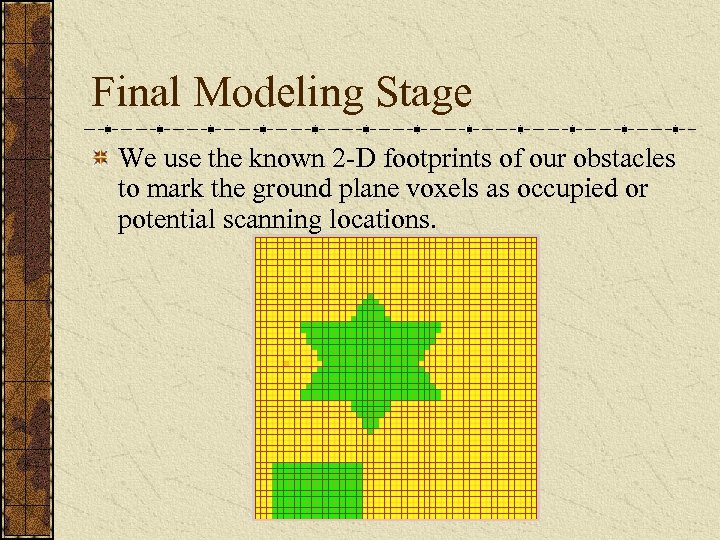
Final Modeling Stage We use the known 2 -D footprints of our obstacles to mark the ground plane voxels as occupied or potential scanning locations.

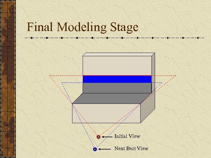
Final Modeling Stage For each unseen voxel that borders on an empty voxel we trace a ray back to all scanning locations. If ray is not occluded by other filled voxels and it satisfies the scanner’s other constraints, that potential viewing location’s counter is incremented. The potential viewing location with the largest count is chosen. A new scan is taken and the process repeats until there are no unseen voxels bordering on empty voxels.

Final Modeling Stage Additional Constraints: Range constraint – the scanner’s minimum and maximum range is considered. If the ray is outside this range, it is not considered. Overlap constraint – for each view we can also keep track of how many known voxels it can view and require a minimum overlap for registration purposes. Traveling distance constraint – weight more heavily views that are closer to the current position. Grazing angle constraint – this constraint is harder to implement since no surface information is stored.

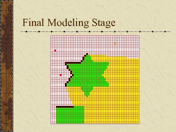
Final Modeling Stage

Final Modeling Stage Initial View Next Best View

Testbeds: Columbia Campus

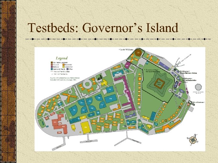
Testbeds: Governor’s Island

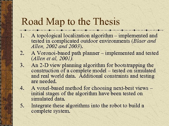
Road Map to the Thesis 1. 2. 3. 4. 5. A topological localization algorithm – implemented and tested in complicated outdoor environments (Blaer and Allen, 2002 and 2003). A Voronoi-based path planner – implemented and tested (Allen et al, 2001). An 2 -D view planning algorithm for bootstrapping the construction of a complete model – tested on simulated and real world data. Additional constraints and testing are needed. A voxel-based method for choosing next-best views – initial stages of the algorithm have been tested on simulated data. Integrate these algorithms into the robot to build a complete system.