Auction Markets Jon Levin Winter 2010 Economics 136

Auction Markets Jon Levin Winter 2010 Economics 136

FCC and Radio Spectrum l FCC regulates use of electromagnetic radio spectrum: used for broadcast TV, radio, cell phones, Wi. Fi, etc. l Why regulate? l There is a limited amount of spectrum l There are many potential users l There are interference problems if users overlap. l So, how should the FCC decide who gets a license to use spectrum? l Historically, licenses were allocated administratively (TV & radio stations) or by lottery.

Spectrum auctions l Coase (1959) suggested that the FCC should auction spectrum licenses. l l l If there were no transaction costs, the initial assignment of ownership wouldn’t matter (the Coase Theorem). But the real world isn’t like that… decentralized trade may not lead to efficient allocations (more on this later). In the early 1990 s, the FCC started to think about auctions as a way to allocate licenses efficiently, and adopted a new design proposed by Stanford economists. l Many countries now use auctions that result in hundreds of millions, or billions, of dollars of government revenue.

Sponsored search auctions l l Google revenue in 2008: $21, 795, 550, 000. Hal Varian, Google chief economist: l l Google revenue comes from selling ads: there is an auction each time someone enters a search query l l l “What most people don’t realize is that all that money comes pennies at a time. ” Bids in the auction determine the ads that appear on the RHS of the page, and sometimes the top. Google design evolved from earlier, and problematic, design used by Overture (now part of Yahoo!) We will see that Google’s design is closely related to theory of matching we’ve already studied.

British CO 2 Auctions l In 2002, the British government decided to spend £ 215 million paying firms to reduce CO 2 emissions. l l l Greenhouse Gas Emissions Trading Scheme Auction l l l But what price to pay per unit? And which firms to reward? Solution: run an auction to find the “market price” Price starts high and decreases each round. Each round, bidders state tons of CO 2 they will abate Cost to UK: tons of abatement times price. Auction ended when total cost equaled the budget. Result: 34 firms paid to reduce emission by a total of 4 million metric tons of CO 2.

Auctions everywhere… l Auctions are commonly used to sell (and buy) goods that are idiosyncratic or hard to price. l l l l Real estate Art, antiques, estates Collectibles (e. Bay) Used cars, equipment Emissions permits Natural resources: timber, gas, oil, radio spectrum… l l Financial assets: treasury bills, corporate debt. Bankruptcy auctions Sale of companies: privatization, IPOs, takeovers, etc. Procurement: highways, construction, defense. Auction theory also has close and beautiful ties to standard price theory (monopoly theory) and matching.

Auction Theory

Selling a single good l We’ll start with sale of a single good (later, consider many goods). l Why not just set a price? l l Potential buyers know what they’d pay, but aren’t telling. l l Seller may not know what price to set. Remember from last time – auction serves as a mechanism for price discovery. Let’s consider different ways to run an auction.

Canonical model l Potential buyers l Two bidders (later N bidders) l Each bidder i has value vi l Each vi drawn from uniform distribution on [0, 1]. l Same ideas will apply with N bidders and a value distribution other than U[0, 1]. l Seller gets to set the auction rules.

Ascending auction l Price starts at zero, and rises slowly. l Buyers indicate their willingness to continue bidding (e. g. keep their hand up) or can exit. l Auction ends when just one bidder remains. l Final bidder wins, and pays the price at which the second remaining bidder dropped out. l How should you bid?

Ascending Auction l Optimal strategy: continue bidding until the price just equals your value. l Bidder with highest value will win. l Winner will pay second highest value. l Example with three bidders l Suppose values are 25, 33, and 75. l First exits at 25, second at 33 and auction ends.

Ascending auction revenue l Suppose we repeatedly take two draws from U[0, 1]. l On average, the highest draw will be 2/3 l On average, the second highest will be 1/3. l So the average (or expected) revenue from an ascending auction with two bidders who have values drawn from U[0, 1] is 1/3. l If we have N bidders with values drawn from U[0, 1] l on average, the highest draw will be N/N+1 l and the second highest draw will be (N-1)/(N+1). l So the expected revenue will be (N-1)/(N+1).

Aside: Order Statistics One draw 0 1 1/2 Two draws 0 1/3 1 2/3 Three draws 0 1/4 2/4 3/4 1

Ascending auction profit l Suppose values are drawn from U[0, 1]. What profit does a bidder with value v expect? l l If he wins, he gets the object worth v l He also pays the highest losing value. l l His probability of winning is v (why? ) If he wins, he expects on average to pay half his value (why? ), or v/2. So average (or expected) profit for value v bidder: v [v-v/2] = v 2[1/2] = (1/2)v 2.

Second price auction l l Bidders submit sealed bids. Seller opens the bids. l l l Bidder who submitted the highest bid wins. Winners pays the second highest bid. How should you bid?

Second price auction Theorem. The optimal strategy in the second price auction is to bid your value. Proof l Suppose you bid b>v. l l l If the highest opposing bid is less than v, or higher than b, it makes no difference. If the highest opposing bid is between v and b; you win if you bid b, but pay above your value, so better to bid v. Suppose you bid b

Second price auction Bid true value v 0 If opponent bid is here, 1 lose the auction If opponent bid is here, win and make money v If bid is b Bid b>v 0 here, win but lose money! If opponent bid is here, lose auction 1

Second price auction l In equilibrium, everyone bids their value. l l l Bidder with highest value wins. Pays an amount equal to second highest value. Exactly the same as the ascending auction! l i. e. same winner, same revenue, same expected profit for a bidder with value v.

Vickrey auction l l Second price auction is an example of a more general “Vickrey” auction that can be used to sell multiple goods. Rules for Vickrey auction (will return to this later) l l l Everyone submits their value(s) Seller allocates to maximize surplus Set prices so the profit of each winner equals his contribution to the total surplus – the difference between social surplus if he is or is not counted as a participant. Equivalently, each winner pays the externality he imposes by displacing other possible winners. Think about how the 2 nd price auction does this!

Sealed tender l l Bidders submit sealed bids. Seller opens the bids and l l l Bidder who submitted highest bid wins. Winner pays his own bid. Now what is the optimal strategy?

Sealed tender, cont. l Best to submit a bid less than your true value. l How much less? l Submitting a higher bid l increases the chance you will win l increases the amount you’ll pay if you do win l Optimal bid depends on what you think the others will bid (unlike in the second-price auction!). l We need to consider an equilibrium analysis.

Nash equilibrium l Defn: A set of bidding strategies is a Nash equilibrium if each bidder’s strategy choice maximizes his payoff given the strategies of the others. l In an auction game, bidders do not know their opponent’s values, i. e. there is incomplete information. l So each bidder’s equilibrium strategy must maximize her expected payoff accounting for the uncertainty about opponent values.

Solving the sealed bid eqm l Suppose j i uses the strategy: bid bj= vj. l l Bidder i understands j’s strategy (the eqm assumption), but doesn’t know j’s bid exactly because he doesn’t know vj. Suppose i bids bi. He’ll win with probability Pr(bi> vj)= Pr(bi/ >vj)= bi/ l So bidder i’s bidding problem is maxb (b/ )(vi-b) l First order condition for optimal bidding 0 = (1/ )(vi-b) – (b/ )

Solving for equilibrium l First order condition 0 = (1/ )(vi-b) – (b/ ) l Re-arranging and cancelling out b/ = (1/ )(vi-b) b = vi-b b =(1/2)v l l At symmetric equilibrium, bi=(1/2)vi, bj=(1/2)vj --both bidders bid half their value. With N bidders, equilibrium is b=[(N-1)/N]v.

Sealed bid equilibrium l We’ve derived the eqm: b(v)=(1/2)v l Bidder with the highest value wins in eqm. l What is the revenue, on average? l Revenue equals bid of the high value bidder l High value, on average, is 2/3 l So highest bid, on average, is 1/3 l Same as the ascending and second price! l Is it the same for each realization of bidder values? l Example: suppose bidder values are ¾ and ½.

Descending price l Price starts high (at least $1). l Price drops slowly (continuously). l At any point, a bidder can claim the item at the current price (and pay that price). l Auction ends as soon as some bidder claims item. l How should you bid?

Descending price l Strategically equivalent to the first price auction! l l Does actually being there make it any different? l No, in both auctions, your bid only matters if you are the winner or tied for winning – a slightly lower bid means paying less if you win, but maybe you lose out. l l Suppose the bidders had to send in computer programs to do the bidding … it would be a 1 st price auction! For any strategies by opponents, bidder i chooses the stopping price (bid) to maximize Pr(win)(v-b) – same problem as in the first price auction. So … eqm strategies in first price and descending auction are the same, and so is expected revenue.

All-pay auction l Bidders submit bids l Seller opens bids l Bidder submitting the highest bid wins l All bidders pay their bids. l How should you bid?

All pay auction l Clearly want to bid less than your value l Bidding more means l l l Greater chance of winning Pay more for sure Suppose we find equilibrium bid strategies. l How will the bids compare to the first-price auction? l Will seller raise more or less revenue in equilibrium?

Comparison of Auctions l At least in our example, a number of standard auctions share the following properties of bidders play according to equilibrium. l l average revenue is the same l l the allocation is efficient average profit of a value v bidder is the same. Next time we’ll explore this result further.

Bidder Strategy

Are bidders really strategic? l Game theory models of auctions assume that bidders understand the environment and behave strategically. A good assumption? l Consider two examples: l l “Skewed bidding” in Forest Service auctions “Excessive bidding” in internet auctions

Scoring rule auctions l l In many auctions, bidders don’t just bid a price, but many prices that are combined into a “score”. The score determines who wins, but the “unit prices” determine the eventual payments. l l l Contractors bid an hourly rate for labor and a cost for materials. Owner picks the bid that appears the most cheapest but actual payment depends on the work done. Firms bidding for timber in the national forests bid a unit price for each species. The prices are multiplied by the estimated quantities to determine the winner. What are the bidders’ incentives?

Timber auction example l Forest Service estimates there are 100 mbf of Douglas Fir and 100 mbf of Western Spruce. l Bidders make “per-unit” bids for Fir and Spruce. l A bidder offers prices of $50 and $60. l Total bid is 100*50 + 100*60 = $11, 000. l High bid wins, but payment depends on actual quantities. l Suppose the ($50, $60) bid wins. l Estimated quantities are 100, 100; expected payment $11, 000. l But if the actual quantities are 100 of fir and 50 of spruce, the actual payment is 100*50 + 50*60 = $8, 000.

Bidding incentives l Suppose FS estimates (100, 100) of fir, spruce. l Bidder can submit a total bid of $10, 000 by: l l Bidding $50 for Fir and $50 for Spruce. Bidding $100 for Fir and $0 for Spruce Bidding $0 for Fir and $100 for Spruce. Suppose bidder estimates (200, 0) for fir, spruce. l l The three alternative bids lead to expected payments of $10, 000, $20, 000, and $0! Incentive to “skew” one’s bid onto the species you think the seller has over-estimated!

Are bids skewed? l l Athey and Levin (2001) show that there is a lot of skewed bidding in Forest Service auctions. FS revenue is about $10, 000 less per sale than if total bids were the same but “balanced”. But, in sales when FS made a mistake, total bids were higher, so there is no correlation between FS mistakes and actual revenue. Explanation? l l Bidders appear to game the auction by making bids for which they expect to pay less. But since they’re all doing it, they have to bid more to win – they compete away the potential profit from gaming!

Overbidding at e. Bay l l Lee and Malmendier (2010) document “excessive” bidding in e. Bay auctions. Look at auctions for a game: Cashflow 101. Available from two e. Bay retailers for $129. 95. Auction prices on e. Bay can exceed this: l l l 42% of auctions in their data! 73% if one accounts for shipping costs. What should we make of this?

Source: Lee and Malmendier (2010)

Overbidding at e. Bay, cont. l Does everyone overbid? l l l How general is the phenomenon? l l Appears to be a small number of bidders: only 17% of bidders ever bid above the retail price. Maybe auctions let you “fish for fools”? Appears to be relatively common in other categories, not a specific “Cashflow 101” effect. So again, what do we make of it?

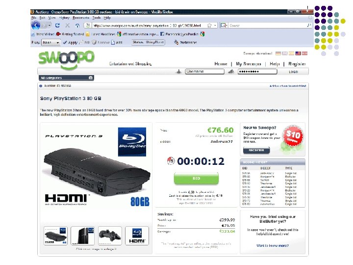
Swoopo Auction l l Swoopo sells common products by auction. Auction rules l l l Placing a bid costs $0. 50. Price starts at $0, and clock starts to run down. If there are bids before clock runs out, new round. In each new round, price increases by $0. 10. If clock expires, auction ends. Standing high bidder is the winner and pays the current price.

Excess Bidding l Data from 650 auctions of $50 bills l l Average revenue: $104! More generally, Augenblick examines data from over 100, 000 Swoopo auctions….

Excessive bidding?

Ending Times: Theory vs Data

Revenue Equivalence

Background l We saw that (in theory) some common auction designs all lead to efficient outcomes and yield the same revenue, at least on average. l Next: l How general is this result? l Why is the case? l What are the implications? l and then a bit of empirical evidence.

Canonical model l Potential buyers l Two bidders. l Bidder i has value vi l Each vi drawn from uniform distribution on [0, 1]. l Our next result also applies with N bidders so long as their values come from the same distribution (doesn’t have to be a uniform distribution). l Seller gets to set the auction rules.

Revenue equivalence theorem Thm. Consider the model on the last slide and any auction game with the feature that in equilibrium, l l the bidder with the highest value wins, and if a bidder has the lowest possible value, he pays nothing. The average revenue and bidder profits in this auction game are the same as in the 2 nd price auction. l Examples: the four main auctions from before l l Ascending auction Second price sealed bid l l Descending auction First price sealed bid

Envelope Theorem l Consider a parameterized maximization problem l Maximization means that when b=b*(v) l By the chain rule for differentiation l The envelope theorem says that

Proof of the RET l l Consider auction game each bidder has to submit a “bid” b. (sealed bid, stopping price. . ) Bidder with value v solves l Let U(v) be the bidder’s expected profit, i. e. the “value” of the bidding problem. The Envelope Theorem says l So the bidder’s expected profit is

Math behind the RET, cont. l So, independent of the exact auction rules (how bids determine the winner and payments), a bidder’s expected profit depends only on his equilibrium probability of winning as a function of his value. l So if some auction game always results in the same allocation (same winner) as the 2 nd auction, it must have the same expected bidder profits. It must also have the same expected revenue. Why? l l Revenue equals the total surplus minus the sum of the bidder profits, and both of these are the same across auctions!

Revenue Equivalence Recap l Bidder values drawn from same distribution. Standard auction with equilibrium in which high value bidder wins. Expect payoff if value v l “Envelope” argument l l l Using calculus l RET: if two auctions would result in the same winner, they have the same bidder profits, and hence seller revenue.

“Hidden” assumptions l Bidders know their own values l l l Bidder values are independent. l l l What if they may want to resell the good? What if another bidder has relevant information? Bidder i and j will have same belief about k’s value. What if bidders conduct surveys of the same oil field? Bidder’s care about their auction profits l l l Value of the object minus the price they pay. If opponent wins, don’t care about what it pays. No “risk aversion” if auction outcome is uncertain.

RET as a benchmark l The revenue equivalence theorem is a central result in auction theory, but it depends on strong assumptions. l Many important results in economics are similar in their dependence on implausible assumptions l l l Modigliani-Miller capital structure theorem Ricardian equivalence theorem First & second welfare theorems Coase theorem What is the significance of these kinds of results?

Evidence on RET

Does the RET Really Hold? l Not in laboratory experiments l l l Bidders behave as predicted in ascending auctions, but tend to bid “too much” in first and second price auctions, and descending auctions! There is some evidence, however, that this goes away with more “experienced” bidders. What about in actual markets?

USFS Timber Auctions l The US Forest Service sells timber from the national forests – sometimes by open auction and sometimes by sealed bid. l Athey, Levin and Seira (2008) use data from these auctions to test predictions of the RET.

Data from Timber Auctions

Empirical Test l Tracts of timber sold by open and sealed bid auction are not identical l l California: small sales are usually sealed and large sales usually open – have to control for auction size. Idaho/Montana: format was partially randomized but varied by location and date of sale – have to control for date/area. Solution: estimate regression model where “outcome” can be participation, revenue, etc.

Estimated effect of sealed bidding Logger More loggers at sealedfor sealed bidding? more likely to win Revenue advantage bid auctions! a sealed bid auction

Explaining the results l Basic RET assumed symmetric bidders, but here we have small “loggers” and large “mills” competing. l What happens with weak and strong bidders? l l l Open auction: outcome is still efficient – high value wins. Sealed auction: strong bidders may “shade” bids a lot, and so weak bidders win more often. So theory predicts weak bidders will do better (attend more, win more) with sealed bidding.

Combining theory and data l Athey-Levin paper asks l l l Suppose mills draw their values from one distribution and loggers from another: what distributions are consistent with the data? Can do this for the open and/or the sealed bid auctions. How do we infer value distributions from bidding data? l One approach: pick a distribution of values, simulate a lot of auctions, see if the simulation data is similar to the actual data; iterate until you find a good fit. l In practice, can be a bit more nuanced.

Findings l California l l The data matches theory very closely. Idaho/Montana l The data doesn’t match theory as wel: the prices in the open auctions are “too low” relative to what theory predicts. l Why? Maybe bidders aren’t competing hard in the open auctions – they bid “as if” they have low values. l Why might open auctions be vulnerable to collusion?

Applying the RET

Applying the RET l The basic idea of the RET is that so long as the equilibrium of the auction leads to the high value bidder winning l l l The bidders will make the same expected profits as in the 2 nd price auction The seller will make the same expected revenue as in the 2 nd price auction Now let’s consider some applications…

Solving the first-price auction l Two bidders and values U[0, 1]. l In a 2 nd price auction, a bidder with value v will win with probability v and expects to pay v/2 when he wins. l Suppose the first price auction has an equilibrium where bidders use an increasing bid strategy b(v), so the high value bidder wins. l A bidder with value v must expect to pay the same as in a 2 nd price auction, i. e. to pay v/2 if he wins. l In the first-price auction, if the winner with value v pays his bid b(v) if he wins, so therefore b(v)=v/2.

All-pay auction l Everyone puts their bid in an envelope and mails the money to the seller. l The seller keeps the bids, and gives the object to the highest bidder. l What are the equilibrium bids? l Suppose there’s an equilibrium in which a higher value leads to a higher bid – then high value bidder will win, and we can use the RET to find out what the bids must be!

Solving the all-pay auction l Two bidders and values U[0, 1]. l In a 2 nd price auction, a bidder with value v will win with probability v and expects to pay v/2 when he wins. l So his overall expected payment is v 2/2. l Suppose the all pay auction has an equilibrium where bidders use an increasing bid strategy b(v), so the high value bidder wins. l A bidder with value v must expect to pay the same as in a 2 nd price auction, i. e. v*v/2=v 2/2 l In the all-pay auction equilibrium, each bidder pays its bid with probability 1, so the bid strategy must be b(v) = v 2/2!

Bidding with Reserve prices l l Again consider two bidders with values U[0, 1]. Consider a second price auction where the seller sets a reserve price r below which she will not sell. l l l A bidder with value below r won’t bid, A bidder with value v>r bids her value. Suppose a bidder has value v>r. l l Expects to win with probability v. Conditional on winning, will pay either r or opponent value. Expects to pay (r/v)*r + [(v-r)/v]*(v+r)/2 if he does win. Re-writing expected payment: r+[(v-r)/v]*(v-r)/2.

First price auction with reserve l Look for an equilibrium where high value bidder wins if his value is above the reserve price. l By RET, in the first price auction equilibrium, l A bidder with vr bids b(v)=r+[(v-r)/v]*(v-r)/2.

Reserve prices and revenue l l l Can a reserve price increase revenue? Suppose there is just one bidder with value v distributed uniformly between 0 and 1. Setting a reserve price r means l l No sale with probability r Sale at price of r with probability 1 -r Want to maximize r(1 -r) => r=1/2! Same as the monopoly price for a seller facing a linear demand curve Q(p)=1 -p. Why?

Reserve prices, cont. l Suppose there are two bidders with values U[0, 1]. l Consider choosing r or slightly more r+ l l l Doesn’t matter if both values above r+ or below r. Increases revenue by if one bidder has value above r+ and one has value below, i. e. with prob. 2 r(1 -r) Decreases revenue by r if one bidder has value between r and r+ , and the other has value below, i. e with prob. 2 r. l At the optimal r, small change can’t matter, so we must have *2 r(1 -r)= r*2 r. l Optimal reserve: r=1/2 – same as with one bidder!

Reserve price and RET l The optimal reserve price is independent of the number of bidders. l And by RET, it’s the same in the first and second price auction (and ascending/descending). l Is it the same in the all-pay auction? l No – but can still use RET logic. l If r* is the optimal reserve in the second-price auction, and b(v) is the all-pay eqm, the optimal all-pay reserve is R*=b(r*).

Buy-it-Now Auctions l l l Two bidders with values U[100, 200] Seller runs ascending auction where bidders can “buy-it-now” at price p. Claim: buy it now will be used at least some of the time if p<50. l l l Suppose opponent never buys it now. If a buyer with value v doesn’t buy it now, he expects to win with prob. (v-100)/200 and pay (100+v)/2, so expected profit (v-100)2/400. Buyer can buy it now for profit v-p, so best to buy-it-now if v -p > (v-100)2/400 – if p=150, buy-it-now if v>158.

Buy-it-Now Auctions l Buy it now equilibrium: each bidder tries to buy it now if v>v*, otherwise waits and bids. l l Here v* is such that v* bidder is just indifferent between buying it now and waiting, given the other bidder tries to buy it now if his v>v*. Claim: introducing “buy it now” reduces profit. l l l With values drawn U[100, 200], MR>0 for all v. So optimal auction awards object to high bidder. May not happen with buy it now: because both bidders may try to buy it now, leading to coin flip!

RET and Bargaining l Consider bargaining situation as follows l l l Seller with value s drawn U[0, 1] Buyer with value v, also drawn from [0, 1]. In a “bargaining protocol”, the seller and buyer report their “bids/offers” – and the mechanism determines whether or not they should trade and who pays/receives what.

Examples l Buyer, seller submit offers b, s (or can opt out) l l l If B, S opt in, trade at price 1/2 (posted price) If b>s, trade at price b (buyer offer ) If b>s, trade at price s (seller offer ) If b>s, trade at price (b+s)/2 (split the difference) If both bid, trade for sure at offer closer to 1/2 (arbitration) Dynamic bargaining l l l Seller and buyer alternate making offers Seller makes offers, buyer says when to accept Actually fits into this framework if we think of bid b and offer s as bargaining strategies rather than numbers.

Vickrey “pivot” mechanism l l l Seller and buyer make bid and ask offers. The parties trade if and only if b>s. If trade takes place, l l The seller receives a price b The buyer pays a price s This mechanism is strategy-proof (optimal to offer true value/cost) and leads to efficient trade. But the payments don’t balance – whenever there is trade, the mechanism requires a subsidy of v-s.

Vickrey mechanism Buyer: bid true value v 0 If seller offer is here, trade at price sv 0 If seller offer is here, trade at price s v! If seller offer is here, don’t trade 1

Cost of Vickrey Mechanism l If v>s, trade occurs l l l Gains from trade v-s Subsidy required is also v-s Expected outcomes l l Expected gains from trade: E[max{v-s, 0}] = 1/6 Expected buyer profit: 1/6 Expected seller profit: 1/6 Expected subsidy: 1/6

Efficiency in Bargaining? l Analogue of the RET for bargaining says that any bargaining protocol that leads to efficient trade must give buyer and seller the same profit they’d get under the Vickrey mechanism. l Theorem. There is no bargaining protocol in that always leads to efficient trade and does not require an external subsidy! l Proof. l Under Vickrey mechanism, expected surplus is E[max{v-s, 0}], buyer profit is E[max{v-s, 0}] and seller profit is E[max{v-s, 0}]. l These numbers are the same in any efficient mechanism. l So buyer and seller profit minus surplus created is E[max{v-s, 0}], which can only happen if there is an outside subsidy!

Auctions vs Bargaining l Recall Coase’s argument for FCC auctions. l l l If licenses are allocated according to some inefficient process, parties may not trade to realize the efficient allocation. Myerson-Satterthwaite Theorem provides a rigorous justification: bargaining with private information is inherently inefficient! But in many cases, it is possible to run an efficient auction (in the symmetric U[0, 1] case, any standard auction will do!).

Optimal Auctions

Optimal auctions l A version of the RET says that the expected revenue from any auction will be the expected marginal revenue from the winning bidder. l The “optimal auction” would award the object to the bidder with highest marginal revenue, conditional on his marginal revenue being positive.

Reserve price example l Two bidders with values U[0, 100] l Define P(q)=100 -100 q l Define MR(q)=100 -200 q l For a given value v, the corresponding “quantity” is the probability of having a value more than v, so MR(v)=100 -2(1 -v/100). l The auction maximizes the seller’s revenue if l The bidder with highest value wins, and the object is awarded if and only v>50. l A first-price auction or a Vickrey auction with reserve price of 50 is revenue-maximizing!

Optimal Auctions l Myerson’s Theorem. Across all auctions, the following achieves the maximum expected revenue: l l Bidders report their values to seller. Bidder with highest MR wins, provided his MR>0. Winner pays an amount equal to the least value he could have reported and still won. Notes l l l Payment rule ensures that auction is strategy-proof. If bidders are symmetric, optimal auction is a standard auction with a reserve price. If asymmetric, optimal auction biases the allocation toward bidders with high MRs, but perhaps lower values.

“Asymmetric” Bidders l Two bidders with values U[20, 60] and U[0, 80] l l l Bidder 1: P(q)=60 -40 q and MR(q)=60 -80 q Bidder 2: P(q)=80 -80 q and MR(q)=80 -160 q Marginal revenue as a function of value l l Bidder 1: MR(v) = 2 v-60 l l If value is v, then q is prob. of higher value. Bidder 2: MR(v) = 2 v-80 Revenue-maximizing auction (picture)

Optimal auction MR Bidder 1 could have lower value, but higher marginal revenue. 80 MR 1(v)=2 v-60 MR 2(v)=2 v-80 40 -40 -80 v 1 v 2* 80 If bidder 1 has value v 1, he wins if v 2 < v 2*! The optimal auction is biased toward bidder one!

Relation to Monopoly Theory l Two Stanford GSB professors, Jeremy Bulow and John Roberts, wrote a famous paper that explained optimal auctions as identical to monopoly pricing. l Each bidder is analagous a separate “market” in which the good can be sold. l Quantity is analogous to probability of winning. l The monopolist can price discriminate, setting different prices in different markets. l Allocating the probability of winning to individual bidders is analogous to allocating quantities across separated markets. l The best strategy for a monopolist is to allocate quantity to the market where marginal revenue is highest, and the same is true for the auctioneer!

Marginal Revenue l There is a useful connection to monopoly theory. l Define a bidder’s “demand” at price p to be the probability his value is above p l Define his inverse demand P(q) to be the price at which there is probabilty q he will buy. l Example, a bidder has value U[20, 60] l l l The bidder’s demand is P(q)=60 -40 q. The “revenue” curve is R(q)=q. P(q)=60 q-40 q 2 Define the bidder’s marginal revenue as d. R(q)/dq. l If values are U[20, 60], MR(q)=60 -80 q.

Marginal Revenue Recap l l From RET analysis, bidder profits and seller revenue are determined by the auction allocation – who wins as a function of the bidder values. Optimal auction design: choose the “revenuemaximizing” allocation rule.

Optimal Auction Design v 2 Efficient allocation: e. g. vickrey auction Bidder 2 wins What happens if bidder 1 wins a bit more often? Bidder 1 wins v 1

Marginal Revenue Recap P Probability bidder would pay a price p defines demand curve for a bidder v P(q) MR(v) 0 MR(v)=marginal revenue from allocating a bit more quantity to the bidder (by letting him win when his value is v-dv rather than just above v) 1 -F(v) 1 MR(q) Q

Optimal Auction Design v 2 What happens if bidder 1 wins a bit more often? For each value v of bidder 1 that gets a little extra chance of winning, seller gains MR 1(v) Bidder 2 wins Bidder 1 wins For each value v of bidder 2 that gets a little less chance of winning, seller loses MR 2(v) v 1

Expected revenue l l Starting from the case where the item is never sold, seller gains MR 1(v) when allocates probabilty to type v of bidder 1, and MR 2(v) when allocates probability to type v of bidder 2. So expected revenue from the auction, is average marginal revenue of the winner!

Optimal Auction Design v 2 Bidder 2 wins Optimal auction awards item to bidder with the higher marginal revenue. MR 1(v 1) =MR 2(v 2) Bidder 1 wins v 1

Optimal Auction Design v 2 Bidder 2 wins MR 1(v 1) =MR 2(v 2)>0 MR 1(v 1)=MR 2(v 2)=0 MR 1(v 1)<0 MR 2(v 2)>0 No sale Reserve price used to ensure no bidder wins with a negative marginal revenue! Bidder 1 wins v 1

Summary l RET is powerful tool for thinking about auctions (or bargaining situations) where bidders have private information. l With symmetric bidders many auctions have the property that l l l In equilibrium, the high value bidder wins. Exp. revenue and bidder profit are identical to a Vickrey auction. Auctioneer may want to distort efficiency to increase revenue l l l Reserve price – even with symmetric bidders Biasing the auction to favor high MR bidders. Concerns we haven’t yet discussed l Getting bidders to show up l Getting bidders to bid competitively

Common Value Auctions

Wallet auction l What’s for sale: the money in my wallet. Second-price auction l How much will you bid? l

Wallet auction l l What’s for sale: the money in my wallet. Second-price auction What if one person gets to look in the wallet. Does this change your bid? Why?

The winner’s curse l l Winning the wallet means that everyone else in the class was more pessimistic about its contents. Winning is “bad news” l l If you had an initial estimate of $100, knowing that everyone else had a lower estimate should cause you to revise your estimate downward. Equilibrium bidding should account for this.

Common value auctions l “Imperfect estimate” model l l l Two bidders with common value v Bidder 1 has estimate s 1 = v+e 1 Bidder 2 has estimate s 2 = v+e 2 Errors e 1, e 2 are independent Second price auction How should bidders account for the winner’s curse in equilibrium?

Equilibrium bidding l Claim: In the equilibrium of the second price auction, bidders use the strategy b(si)=E[v|si, sj=si] l Proof. l l Suppose b(s) is an equilibrium bid strategy. Then i prefers to bid “as if” his value is si as opposed to si-ds or si+ds. Changing the bid a little will matter if and only if bidder j bids exactly b(si), that is, if j has the same value. In order that i not want to slightly raise or lower his bid, winning and finding out that j has exactly the same value must result in zero profit. Therefore b(si)=E[v|si, sj=si].

Winner’s or Loser’s Curse? l Does accounting for the information of other’s mean you bid higher or lower than your baseline estimate? l Case 1: 10 bidders, 1 item, second price auction. l l l Eqm: b(s) = E[v|s is tied for highest estimate] < E[v|s]. There is a winner’s curse. Case 2: 10 bidders, 8 items, ninth price auction. l Eqm: b(s) = E[v|s is tied for eigth highest estimate] > E[v|s] l There is a loser’s curse!

Revenue Equivalence? l Milgrom-Weber: If bidders have “correlated” estimates of a common value item, an open auction leads to higher revenue than sealed bid auction. l Intuition. l l l In either case, the high estimate bidder will win. In first price sealed bid auction, the payment will be independent of the estimate of the second highest bidder. In an ascending auction, the payment will depend on the second highest estimate. The bidder estimates are correlated. So open auction sets the price for the winner high when the other bidder has good new about the value, and sets it low when the other bidder has bad news. This reduces the winner’s profit and increases revenue!

“Linkage principle” l Broader principle: suppose the seller can give bidders access to better information. Then revenue is increased on average by making the information publicly available. l Intuition: l The public information can either increase or decrease everyone’s bids (depending on if it’s good or bad news). l The public information will tend to be good news exactly when the high bidder has a high value. l So releasing information “squeezes” the high bidder in the right cases.

Information aggregation l How many miles is it to drive from New York to Chicago?

Information aggregation l Suppose we have many bidders, and each has an independent estimate si = v+ei. l Average of the bidder’s estimates si is likely to be a very good estimate of v. Why? Avg(si) = Avg(v+ei) = v+Avg(ei) ≈ v. l “The wisdom of crowds”; Galton example.

Information aggregation l Suppose we have many bidders, and each has an independent estimate si = v+ei. l If the bidders compete in a (first or second price or ascending) auction, is the resulting price a good estimate of v? l l Answer of Stanford profs Wilson, Milgrom In certain cases YES!, auction prices aggregate information.

Information Aggregation l l In certain cases, auction prices aggregate information, so that the auction price is a “good” estimate of true value. Why? Example: l l l Bidder estimates are si = v+ei. Second price auction, bi = E[v| si is tied for high s] Order bids so that b 1 >b 2 > … >b. N Price = b 2 = E[v| s 2 is tied for high s] With many bidders then “s 2 is tied for high s” is basically a correct hypothesis, so b 2 is an accurate estimate! There is one hidden assumption, which bidders with very extreme estimates are in fact quite confident about the value.

Information Aggregation Signals if true value is low Signals if true value is high Very high signal is very informative! This signal is also very informative if you assume it’s highest.

Common values in practice l What kinds of auction have a “common value” flavor to them? l Treasury bill auctions or other financial assets – everyone may have a guess about the trading price after the auction, but no one knows for sure. l Timber auctions? what kind of timber is actually out there on the tract that’s being sold. l Oil lease auctions: oil is under the Gulf of Mexico, bidders do independent seismic studies – each has valuable information.

OCS Auctions l l The US government auctions the right to drill for oil on the outer continental shelf. Value of oil is similar to the different bidders, but no one knows how much oil there is, or if there’s none. Prior to the auction, the bidders do seismic studies. Two kinds of sale l l l “Wildcat sale” - new territory being sold “Drainage sale” - territory adjacent to existing tract. These are like the “wallet auctions” we ran in class!

Wildcat vs Drainage

Drainage sales

Explaining the Results l Comparing wildcat and drainage sales l l l Wildcat sales yield low profits => competition. Drainage sales are profitable, but only for “insiders” => insiders have an advantage. Next slides (which we won’t cover today) work out equilibrium bidding for an “insider/outsider” model. l l This model fits the drainage data quite well. The symmetric model fits the wildcat data!

Drainage sales l Asymmetric information model l l Neighbor knows true value v. Outsider believes v is U[0, 1]. In ascending auction, outsider drops out at zero! What about first price sealed bid auction? Captures the idea that the bidder with the neighboring tract has superior information.

Bidding in drainage model l There is no equilibrium in which the outsider uses a “pure” strategy. l Suppose the neighbor expects the outsider to bid b. l Neighbor will bid b if b>v, or else less than b. l So the outsider wins and pays b if and only if v0 can’t be optimal, and there can’t be an equilibrium in which the outsider bids b>0 for sure. l There also can’t be an equilibrium with b=0. The neighbor would also bid zero (or epsilon), and the outsider could profitably bid just a bit more and win for sure.

Mixed strategy equilibrium l In equilibrium, the outsider randomizes between different bids – each bid gives him an expected payoff of zero. l l l Outsider bids less than x with probability P(x)=2 x. Neighbor bids b(v)=v/2 if value is v. Features of the equilibrium l Bids of both bidders are uniformly distributed on [0, 1/2]. l The neighbor wins exactly half the time, but tends to win when v is high, and makes positive profit. The outsider also wins half the time, but makes zero profit on average. l

Verifying the equilibrium l Outsider profit (equals zero for all bids x) l l Define g(x)=b-1(x): (x)=Pr(v

Verifying the equilibrium l Neighbor’s problem l l l Given v, choose bid b to maximize P(b)(b-v) Neighbor’s first order condition: b=v-P(b)/P’(b) But we know b(v)=v/2, so therefore P(b)=2 b.

Testing equal distributions

Summary l Many auctions have a “common value flavor. l In common value auctions l l l Auctions that aggregate participant information into the price can yield more revenue. If there are many bidders, the resulting price can be a useful indicator of the item’s value. The distribution of information is very important.