c81d8f851745e7360bc457d6d246503b.ppt
- Количество слайдов: 58
 Association Rules: Advanced Topics
 Apriori Adv/Disadv • Advantages: – Uses large itemset property. – Easily parallelized – Easy to implement. • Disadvantages: – Assumes transaction database is memory resident. – Requires up to m database scans.
 Vertical Layout • Rather than have – Transaction ID – list of items (Transactional) • We have – Item – List of transactions (TID-list) • Now to count itemset AB – Intersect TID-list of item. A with TID-list of item. B • All data for a particular item is available
 Eclat Algorithm • Dynamically process each transaction online maintaining 2 -itemset counts. • Transform – Partition L 2 using 1 -item prefix • Equivalence classes - {AB, AC, AD}, {BC, BD}, {CD} – Transform database to vertical form • Asynchronous Phase – For each equivalence class E • Compute frequent (E)
 Asynchronous Phase • Compute Frequent (E_k-1) – For all itemsets I 1 and I 2 in E_k-1 • If (I 1 ∩ I 2 >= minsup) add I 1 and I 2 to L_k – Partition L_k into equivalence classes – For each equivalence class E_k in L_k • Compute_frequent (E_k) • Properties of ECLAT – Locality enhancing approach – Easy and efficient to parallelize – Few scans of database (best case 2)
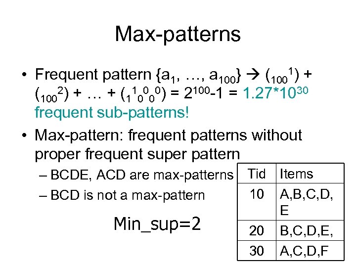 Max-patterns • Frequent pattern {a 1, …, a 100} (1001) + (1002) + … + (110000) = 2100 -1 = 1. 27*1030 frequent sub-patterns! • Max-pattern: frequent patterns without proper frequent super pattern – BCDE, ACD are max-patterns Tid Items 10 A, B, C, D, – BCD is not a max-pattern E Min_sup=2 20 B, C, D, E, 30 A, C, D, F
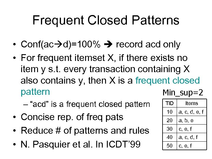 Frequent Closed Patterns • Conf(ac d)=100% record acd only • For frequent itemset X, if there exists no item y s. t. every transaction containing X also contains y, then X is a frequent closed pattern Min_sup=2 – “acd” is a frequent closed pattern • Concise rep. of freq pats • Reduce # of patterns and rules • N. Pasquier et al. In ICDT’ 99 TID Items 10 a, c, d, e, f 20 a, b, e 30 c, e, f 40 a, c, d, f 50 c, e, f
 Mining Various Kinds of Rules or Regularities • Multi-level, quantitative association rules, correlation and causality, ratio rules, sequential patterns, emerging patterns, temporal associations, partial periodicity • Classification, clustering, iceberg cubes, etc.
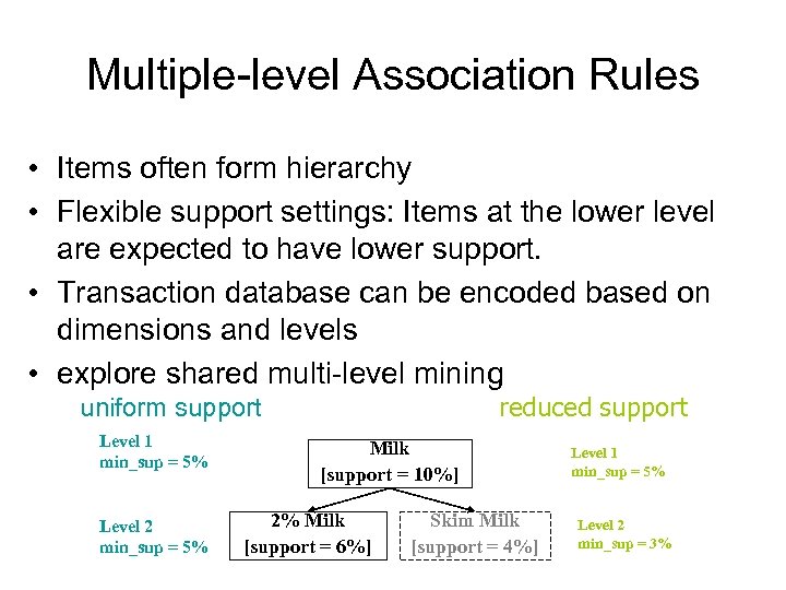 Multiple-level Association Rules • Items often form hierarchy • Flexible support settings: Items at the lower level are expected to have lower support. • Transaction database can be encoded based on dimensions and levels • explore shared multi-level mining reduced support uniform support Level 1 min_sup = 5% Level 2 min_sup = 5% Milk [support = 10%] 2% Milk [support = 6%] Skim Milk [support = 4%] Level 1 min_sup = 5% Level 2 min_sup = 3%
 ML/MD Associations with Flexible Support Constraints • Why flexible support constraints? – Real life occurrence frequencies vary greatly • Diamond, watch, pens in a shopping basket – Uniform support may not be an interesting model • A flexible model – The lower-level, the more dimension combination, and the long pattern length, usually the smaller support – General rules should be easy to specify and understand – Special items and special group of items may be specified individually and have higher priority
 Multi-dimensional Association • Single-dimensional rules: buys(X, “milk”) buys(X, “bread”) • Multi-dimensional rules: 2 dimensions or predicates – Inter-dimension assoc. rules (no repeated predicates) age(X, ” 19 -25”) occupation(X, “student”) buys(X, “coke”) – hybrid-dimension assoc. rules (repeated predicates) age(X, ” 19 -25”) buys(X, “popcorn”) buys(X, “coke”)
 Multi-level Association: Redundancy Filtering • Some rules may be redundant due to “ancestor” relationships between items. • Example – milk wheat bread [support = 8%, confidence = 70%] – 2% milk wheat bread [support = 2%, confidence = 72%] • We say the first rule is an ancestor of the second rule. • A rule is redundant if its support is close to the “expected” value, based on the rule’s ancestor.
 Multi-Level Mining: Progressive Deepening • A top-down, progressive deepening approach: – First mine high-level frequent items: milk (15%), bread (10%) – Then mine their lower-level “weaker” frequent itemsets: 2% milk (5%), wheat bread (4%) • Different min_support threshold across multilevels lead to different algorithms: – If adopting the same min_support across multi-levels then toss t if any of t’s ancestors is infrequent. – If adopting reduced min_support at lower levels then examine only those descendents whose ancestor’s
![Interestingness Measure: Correlations (Lift) • play basketball eat cereal [40%, 66. 7%] is misleading Interestingness Measure: Correlations (Lift) • play basketball eat cereal [40%, 66. 7%] is misleading](https://present5.com/presentation/c81d8f851745e7360bc457d6d246503b/image-14.jpg) Interestingness Measure: Correlations (Lift) • play basketball eat cereal [40%, 66. 7%] is misleading – The overall percentage of students eating cereal is 75% which is higher than 66. 7%. • play basketball not eat cereal [20%, 33. 3%] is more accurate, although with lower support and confidence • Measure of dependent/correlated events: lift Basketbal Not basketball l Sum (row) Cereal 2000 1750 3750 Not cereal 1000 250 1250 Sum(col. ) 3000 2000 5000
Interestingness Measure: Correlations (Lift) • play basketball eat cereal [40%, 66. 7%] is misleading – The overall percentage of students eating cereal is 75% which is higher than 66. 7%. • play basketball not eat cereal [20%, 33. 3%] is more accurate, although with lower support and confidence • Measure of dependent/correlated events: lift Basketbal Not basketball l Sum (row) Cereal 2000 1750 3750 Not cereal 1000 250 1250 Sum(col. ) 3000 2000 5000
 Constraint-based Data Mining • Finding all the patterns in a database autonomously? — unrealistic! – The patterns could be too many but not focused! • Data mining should be an interactive process – User directs what to be mined using a data mining query language (or a graphical user interface) • Constraint-based mining – User flexibility: provides constraints on what to be mined – System optimization: explores such constraints for efficient mining—constraint-based mining
 Constrained Frequent Pattern Mining: A Mining Query Optimization Problem • Given a frequent pattern mining query with a set of constraints C, the algorithm should be – sound: it only finds frequent sets that satisfy the given constraints C – complete: all frequent sets satisfying the given constraints C are found • A naïve solution – First find all frequent sets, and then test them for constraint satisfaction • More efficient approaches: – Analyze the properties of constraints comprehensively – Push them as deeply as possible inside the frequent pattern computation.
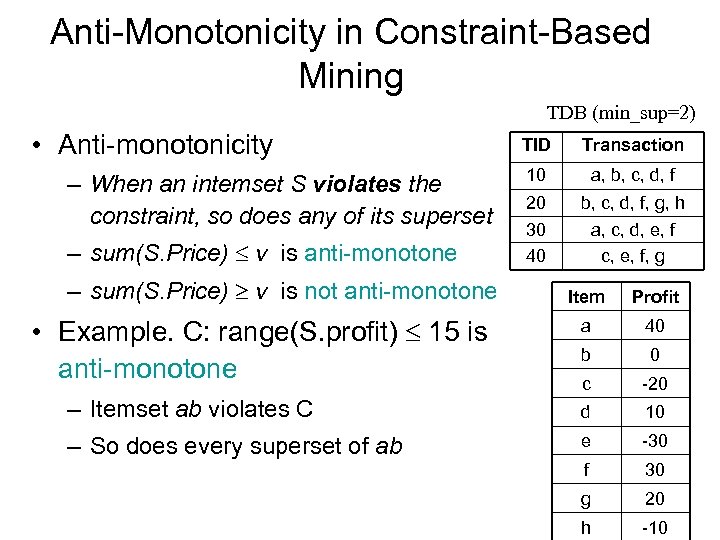 Anti-Monotonicity in Constraint-Based Mining TDB (min_sup=2) • Anti-monotonicity – When an intemset S violates the constraint, so does any of its superset – sum(S. Price) v is anti-monotone – sum(S. Price) v is not anti-monotone TID Transaction 10 a, b, c, d, f 20 30 40 b, c, d, f, g, h a, c, d, e, f c, e, f, g Item Profit a 40 b 0 c -20 – Itemset ab violates C d 10 – So does every superset of ab e -30 f 30 g 20 h -10 • Example. C: range(S. profit) 15 is anti-monotone
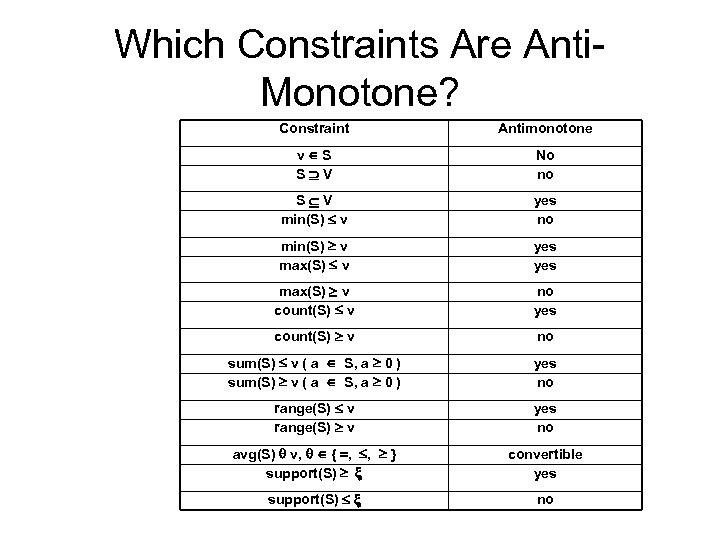 Which Constraints Are Anti. Monotone? Constraint Antimonotone v S S V No no S V min(S) v yes no min(S) v max(S) v yes max(S) v count(S) v no yes count(S) v no sum(S) v ( a S, a 0 ) yes no range(S) v yes no avg(S) v, { , , } support(S) convertible yes support(S) no
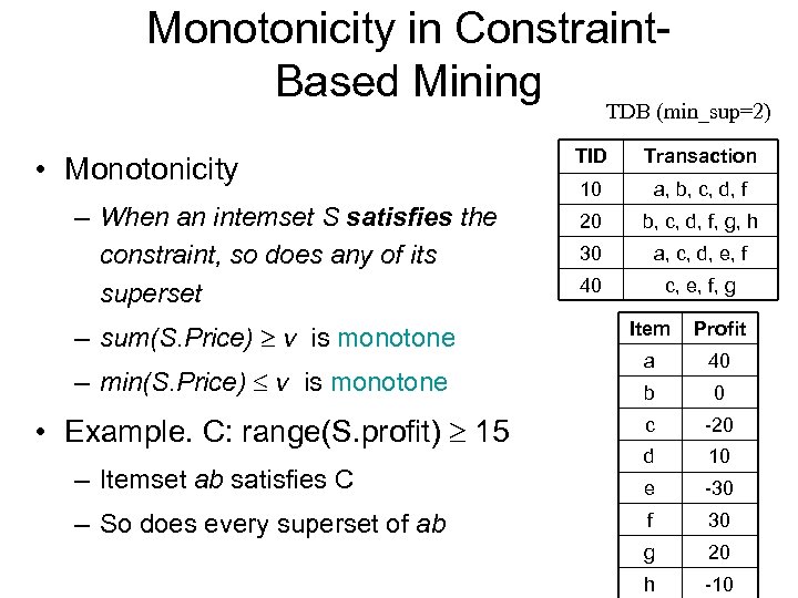 Monotonicity in Constraint. Based Mining TDB (min_sup=2) • Monotonicity – When an intemset S satisfies the constraint, so does any of its superset – sum(S. Price) v is monotone – min(S. Price) v is monotone • Example. C: range(S. profit) 15 – Itemset ab satisfies C – So does every superset of ab TID Transaction 10 a, b, c, d, f 20 b, c, d, f, g, h 30 a, c, d, e, f 40 c, e, f, g Item Profit a 40 b 0 c -20 d 10 e -30 f 30 g 20 h -10
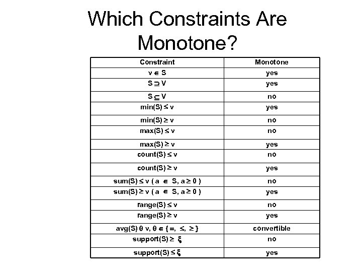 Which Constraints Are Monotone? Constraint v S S V Monotone yes S V min(S) v no yes min(S) v max(S) v no no max(S) v count(S) v yes no count(S) v yes sum(S) v ( a S, a 0 ) no yes range(S) v no yes avg(S) v, { , , } support(S) convertible no support(S) yes
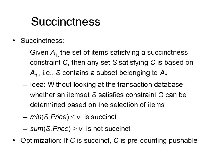 Succinctness • Succinctness: – Given A 1, the set of items satisfying a succinctness constraint C, then any set S satisfying C is based on A 1 , i. e. , S contains a subset belonging to A 1 – Idea: Without looking at the transaction database, whether an itemset S satisfies constraint C can be determined based on the selection of items – min(S. Price) v is succinct – sum(S. Price) v is not succinct • Optimization: If C is succinct, C is pre-counting pushable
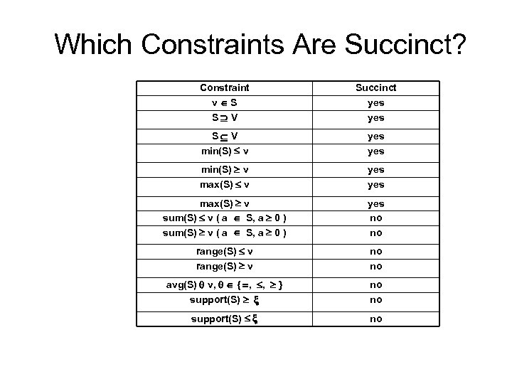 Which Constraints Are Succinct? Constraint v S S V Succinct yes S V min(S) v yes min(S) v max(S) v yes max(S) v sum(S) v ( a S, a 0 ) yes no no range(S) v no no avg(S) v, { , , } support(S) no no support(S) no
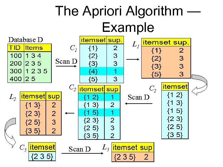 The Apriori Algorithm — Example Database D L 1 C 1 Scan D C 2 Scan D L 2 C 3 Scan D L 3
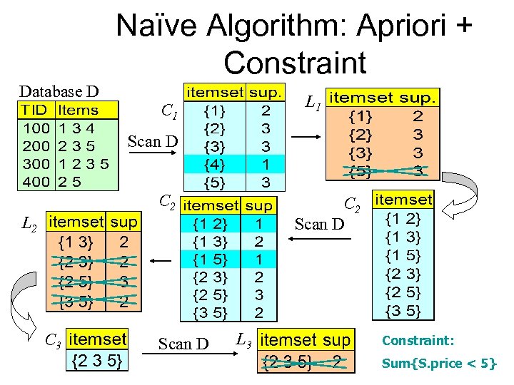 Naïve Algorithm: Apriori + Constraint Database D L 1 C 1 Scan D C 2 Scan D L 2 C 3 Scan D L 3 Constraint: Sum{S. price < 5}
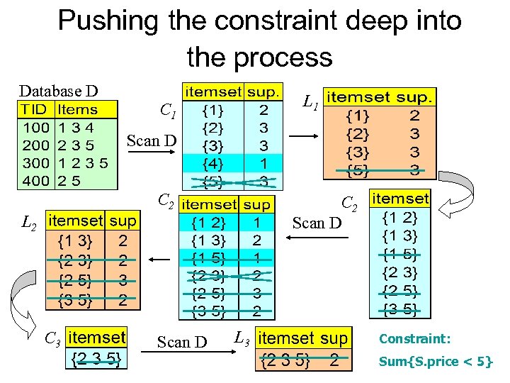 Pushing the constraint deep into the process Database D L 1 C 1 Scan D C 2 Scan D L 2 C 3 Scan D L 3 Constraint: Sum{S. price < 5}
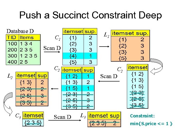 Push a Succinct Constraint Deep Database D L 1 C 1 Scan D C 2 Scan D L 2 C 3 Scan D L 3 Constraint: min{S. price <= 1 }
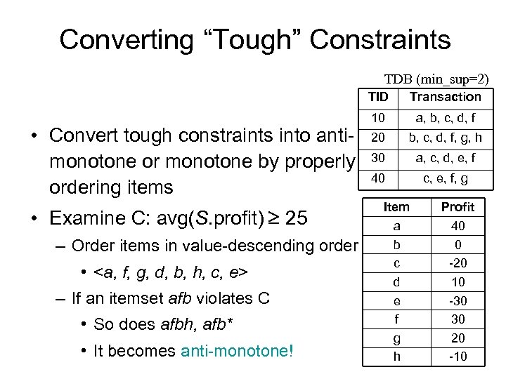 Converting “Tough” Constraints TDB (min_sup=2) TID • Convert tough constraints into antimonotone or monotone by properly ordering items • Examine C: avg(S. profit) 25 – Order items in value-descending order •
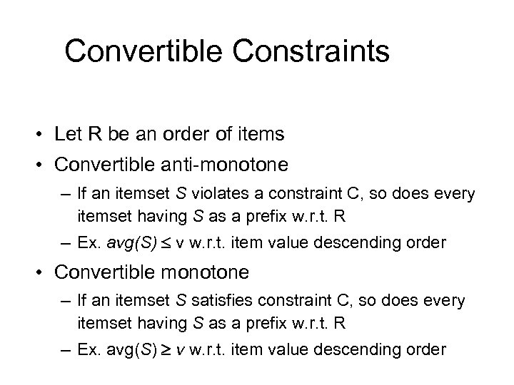 Convertible Constraints • Let R be an order of items • Convertible anti-monotone – If an itemset S violates a constraint C, so does every itemset having S as a prefix w. r. t. R – Ex. avg(S) v w. r. t. item value descending order • Convertible monotone – If an itemset S satisfies constraint C, so does every itemset having S as a prefix w. r. t. R – Ex. avg(S) v w. r. t. item value descending order
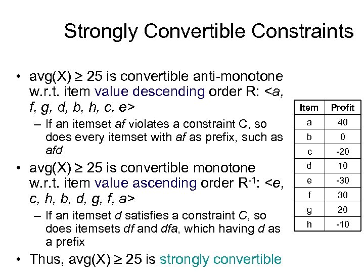 Strongly Convertible Constraints • avg(X) 25 is convertible anti-monotone w. r. t. item value descending order R:
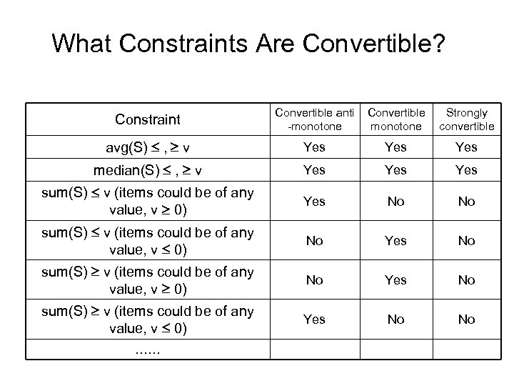 What Constraints Are Convertible? Constraint Convertible anti -monotone Convertible monotone Strongly convertible avg(S) , v Yes Yes median(S) , v Yes Yes sum(S) v (items could be of any value, v 0) Yes No No sum(S) v (items could be of any value, v 0) No Yes No sum(S) v (items could be of any value, v 0) Yes No No ……
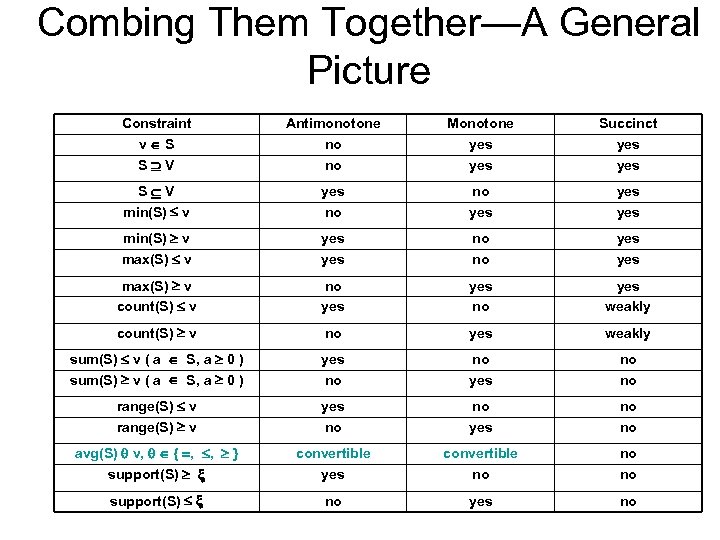 Combing Them Together—A General Picture Constraint v S S V Antimonotone no no Monotone yes Succinct yes S V min(S) v yes no no yes yes min(S) v max(S) v yes no no yes max(S) v count(S) v no yes weakly count(S) v no yes weakly sum(S) v ( a S, a 0 ) yes no no range(S) v yes no no avg(S) v, { , , } support(S) convertible yes convertible no no no support(S) no yes no
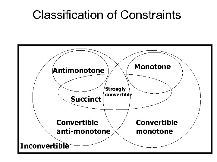 Classification of Constraints Monotone Antimonotone Succinct Strongly convertible Convertible anti-monotone Inconvertible Convertible monotone
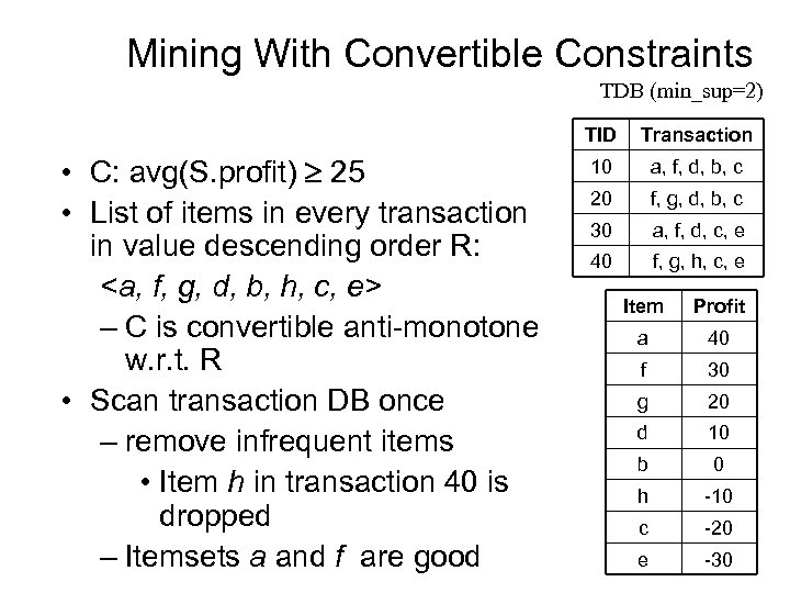 Mining With Convertible Constraints TDB (min_sup=2) TID • C: avg(S. profit) 25 • List of items in every transaction in value descending order R:
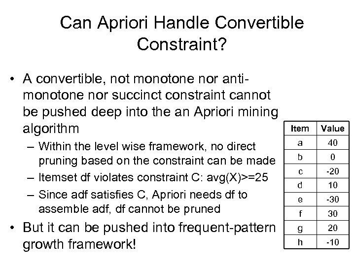 Can Apriori Handle Convertible Constraint? • A convertible, not monotone nor antimonotone nor succinct constraint cannot be pushed deep into the an Apriori mining algorithm Item Value – Within the level wise framework, no direct pruning based on the constraint can be made – Itemset df violates constraint C: avg(X)>=25 – Since adf satisfies C, Apriori needs df to assemble adf, df cannot be pruned a 40 b 0 c -20 d 10 e -30 f 30 • But it can be pushed into frequent-pattern growth framework! g 20 h -10
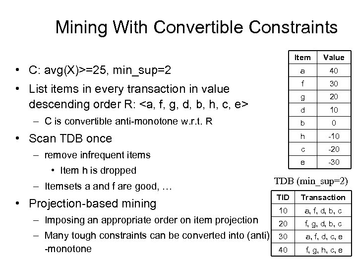 Mining With Convertible Constraints Item Value • C: avg(X)>=25, min_sup=2 a 40 • List items in every transaction in value descending order R:
 Handling Multiple Constraints • Different constraints may require different or even conflicting item-ordering • If there exists an order R s. t. both C 1 and C 2 are convertible w. r. t. R, then there is no conflict between the two convertible constraints • If there exists conflict on order of items – Try to satisfy one constraint first – Then using the order for the other constraint to
 Sequence Mining
 Sequence Databases and Sequential Pattern Analysis • Transaction databases, time-series databases vs. sequence databases • Frequent patterns vs. (frequent) sequential patterns • Applications of sequential pattern mining – Customer shopping sequences: • First buy computer, then CD-ROM, and then digital camera, within 3 months. – Medical treatment, natural disasters (e. g. , earthquakes), science & engineering processes, stocks and markets, etc. – Telephone calling patterns, Weblog click streams – DNA sequences and gene structures
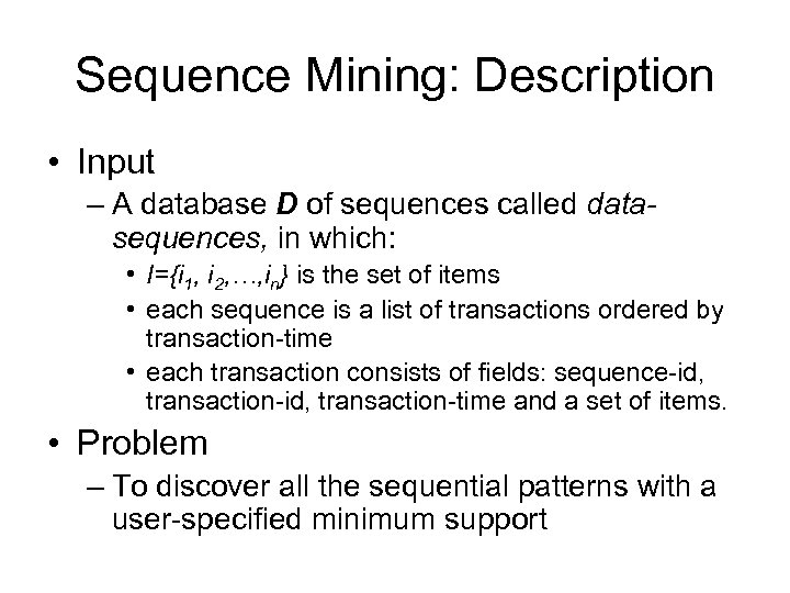 Sequence Mining: Description • Input – A database D of sequences called datasequences, in which: • I={i 1, i 2, …, in} is the set of items • each sequence is a list of transactions ordered by transaction-time • each transaction consists of fields: sequence-id, transaction-time and a set of items. • Problem – To discover all the sequential patterns with a user-specified minimum support
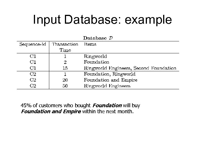 Input Database: example 45% of customers who bought Foundation will buy Foundation and Empire within the next month.
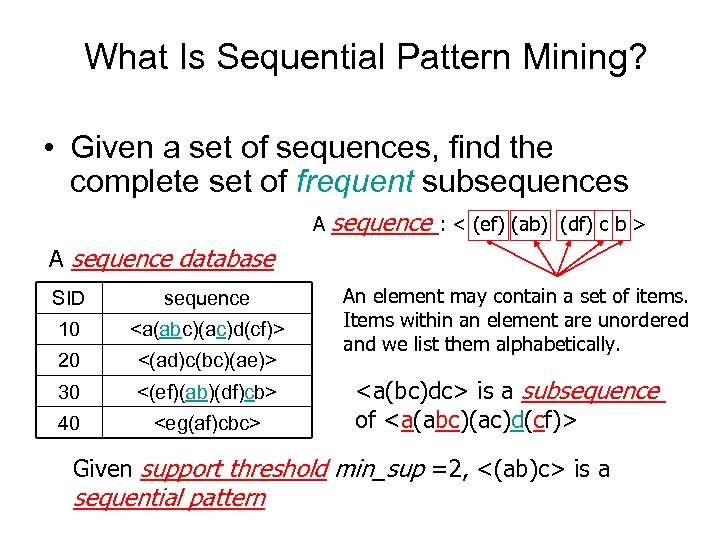 What Is Sequential Pattern Mining? • Given a set of sequences, find the complete set of frequent subsequences A sequence : < (ef) (ab) (df) c b > A sequence database SID sequence 10
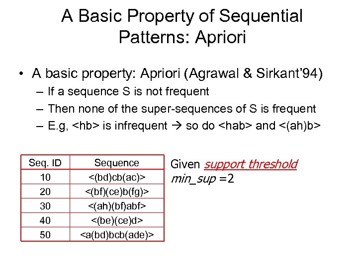 A Basic Property of Sequential Patterns: Apriori • A basic property: Apriori (Agrawal & Sirkant’ 94) – If a sequence S is not frequent – Then none of the super-sequences of S is frequent – E. g,
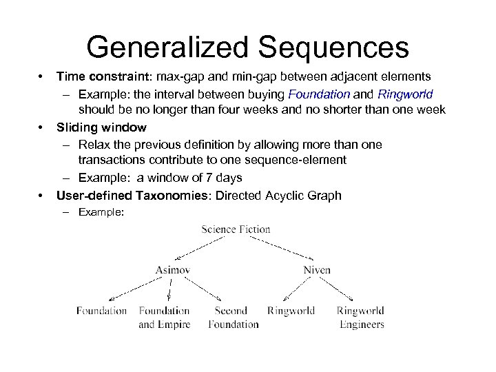 Generalized Sequences • • • Time constraint: max-gap and min-gap between adjacent elements – Example: the interval between buying Foundation and Ringworld should be no longer than four weeks and no shorter than one week Sliding window – Relax the previous definition by allowing more than one transactions contribute to one sequence-element – Example: a window of 7 days User-defined Taxonomies: Directed Acyclic Graph – Example:
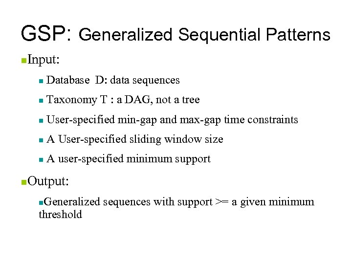 GSP: Generalized Sequential Patterns n Input: n n Taxonomy T : a DAG, not a tree n User-specified min-gap and max-gap time constraints n A User-specified sliding window size n n Database D: data sequences A user-specified minimum support Output: Generalized sequences with support >= a given minimum threshold n
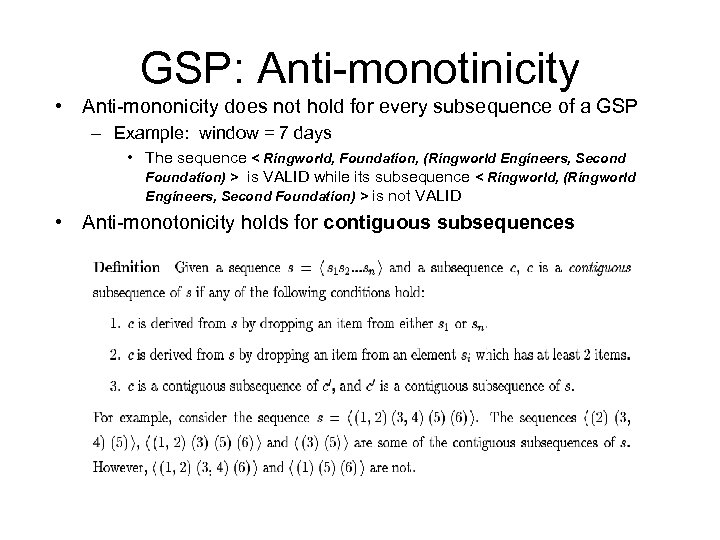 GSP: Anti-monotinicity • Anti-mononicity does not hold for every subsequence of a GSP – Example: window = 7 days • The sequence < Ringworld, Foundation, (Ringworld Engineers, Second Foundation) > is VALID while its subsequence < Ringworld, (Ringworld Engineers, Second Foundation) > is not VALID • Anti-monotonicity holds for contiguous subsequences
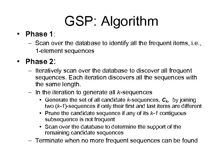 GSP: Algorithm • Phase 1: – Scan over the database to identify all the frequent items, i. e. , 1 -element sequences • Phase 2: – Iteratively scan over the database to discover all frequent sequences. Each iteration discovers all the sequences with the same length. – In the iteration to generate all k-sequences • Generate the set of all candidate k-sequences, Ck, by joining two (k-1)-sequences if only their first and last items are different • Prune the candidate sequence if any of its k-1 contiguous subsequence is not frequent • Scan over the database to determine the support of the remaining candidate sequences – Terminate when no more frequent sequences can be found
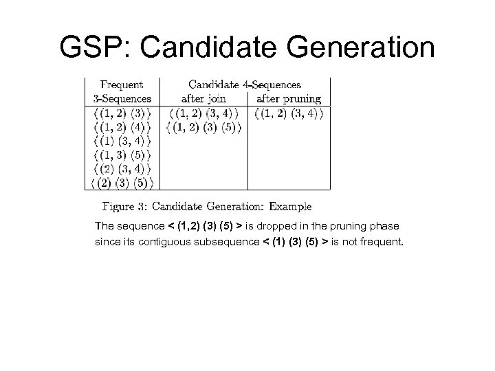 GSP: Candidate Generation The sequence < (1, 2) (3) (5) > is dropped in the pruning phase since its contiguous subsequence < (1) (3) (5) > is not frequent.
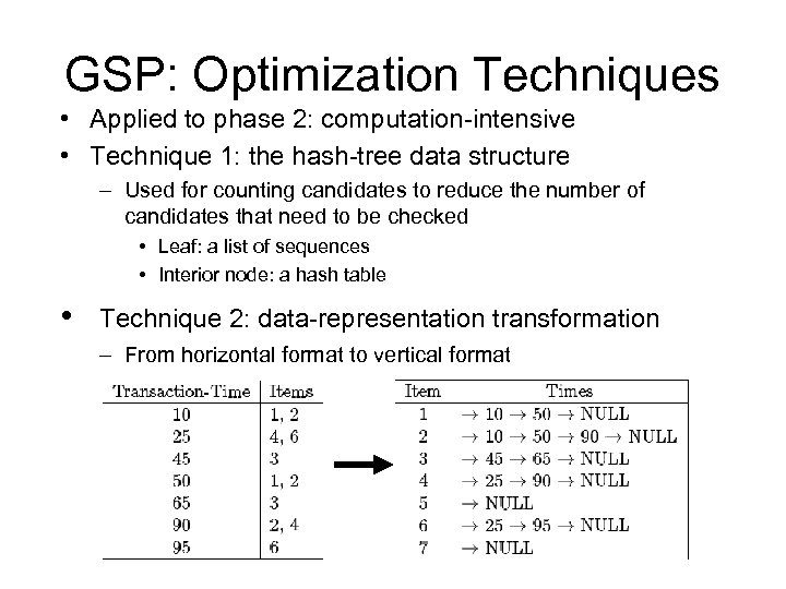 GSP: Optimization Techniques • Applied to phase 2: computation-intensive • Technique 1: the hash-tree data structure – Used for counting candidates to reduce the number of candidates that need to be checked • Leaf: a list of sequences • Interior node: a hash table • Technique 2: data-representation transformation – From horizontal format to vertical format
 GSP: plus taxonomies • Naïve method: post-processing • Extended data-sequences – Insert all the ancestors of an item to the original transaction – Apply GSP • Redundant sequences – A sequence is redundant if its actual support is close to its expected support
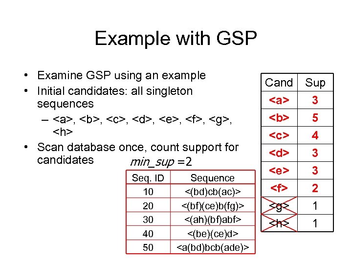 Example with GSP • Examine GSP using an example • Initial candidates: all singleton sequences – , ,
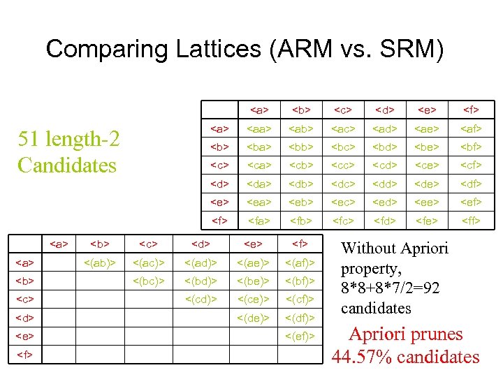 Comparing Lattices (ARM vs. SRM)
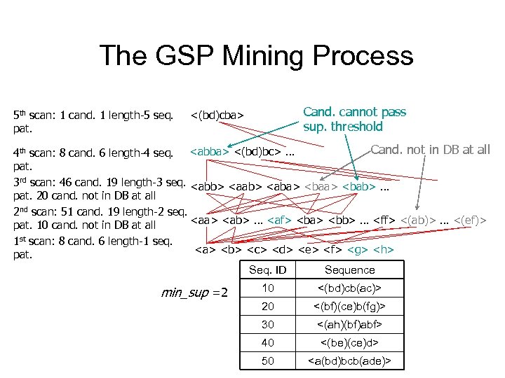 The GSP Mining Process 5 th scan: 1 cand. 1 length-5 seq. pat. Cand. cannot pass sup. threshold <(bd)cba> Cand. not in DB at all 4 th scan: 8 cand. 6 length-4 seq.
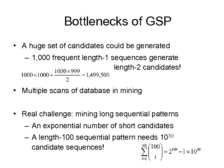 Bottlenecks of GSP • A huge set of candidates could be generated – 1, 000 frequent length-1 sequences generate length-2 candidates! • Multiple scans of database in mining • Real challenge: mining long sequential patterns – An exponential number of short candidates – A length-100 sequential pattern needs 1030 candidate sequences!
 SPADE • Problems in the GSP Algorithm – Multiple database scans – Complex hash structures with poor locality – Scale up linearly as the size of dataset increases • SPADE: Sequential PAttern Discovery using Equivalence classes – Use a vertical id-list database – Prefix-based equivalence classes – Frequent sequences enumerated through simple temporal joins – Lattice-theoretic approach to decompose search space • Advantages of SPADE – 3 scans over the database – Potential for in-memory computation and parallelization
 Recent studies: Mining Constrained Sequential patterns • Naïve method: constraints as a postprocessing filter – Inefficient: still has to find all patterns • How to push various constraints into the mining systematically?
 Examples of Constraints • Item constraint – Find web log patterns only about online-bookstores • Length constraint – Find patterns having at least 20 items • Super pattern constraint – Find super patterns of “PC digital camera” • Aggregate constraint – Find patterns that the average price of items is over $100
 Characterizations of Constraints • SOUND FAMILIAR ? • Anti-monotonic constraint – If a sequence satisfies C so does its non-empty subsequences – Examples: support of an itemset >= 5% • Monotonic constraint – If a sequence satisfies C so does its super sequences – Examples: len(s) >= 10 • Succinct constraint – Patterns satisfying the constraint can be constructed systematically according to some rules • Others: the most challenging!!
 Covered in Class Notes (not available in slide form Scalable extensions to FPM algorithms – Partition I/O – Distributed (Parallel) Partition I/O – Sampling-based ARM


