6d1749c2eedc1b9056679efb698c4f64.ppt
- Количество слайдов: 70
Association Analysis: Basic Concepts and Algorithms 1
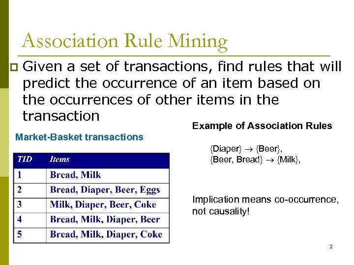
Association Rule Mining p Given a set of transactions, find rules that will predict the occurrence of an item based on the occurrences of other items in the transaction Example of Association Rules Market-Basket transactions {Diaper} {Beer}, {Beer, Bread} {Milk}, Implication means co-occurrence, not causality! 2
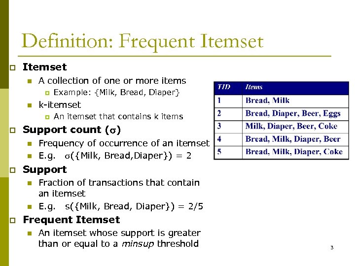
Definition: Frequent Itemset p Itemset n A collection of one or more items p n k-itemset p p n Frequency of occurrence of an itemset E. g. ({Milk, Bread, Diaper}) = 2 Support n n p An itemset that contains k items Support count ( ) n p Example: {Milk, Bread, Diaper} Fraction of transactions that contain an itemset E. g. s({Milk, Bread, Diaper}) = 2/5 Frequent Itemset n An itemset whose support is greater than or equal to a minsup threshold 3
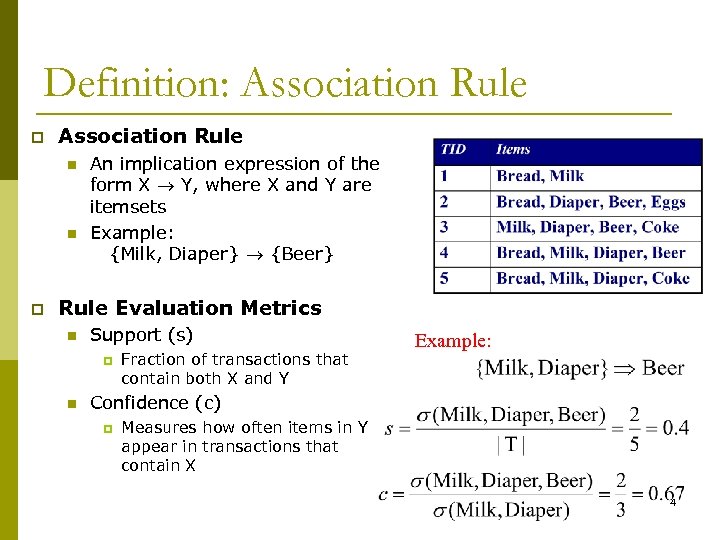
Definition: Association Rule p Association Rule n n p An implication expression of the form X Y, where X and Y are itemsets Example: {Milk, Diaper} {Beer} Rule Evaluation Metrics n Support (s) p n Fraction of transactions that contain both X and Y Example: Confidence (c) p Measures how often items in Y appear in transactions that contain X 4
Association Rule Mining Task p Given a set of transactions T, the goal of association rule mining is to find all rules having n n p support ≥ minsup threshold confidence ≥ minconf threshold Brute-force approach: List all possible association rules n Compute the support and confidence for each rule n Prune rules that fail the minsup and minconf thresholds Computationally prohibitive! n 5
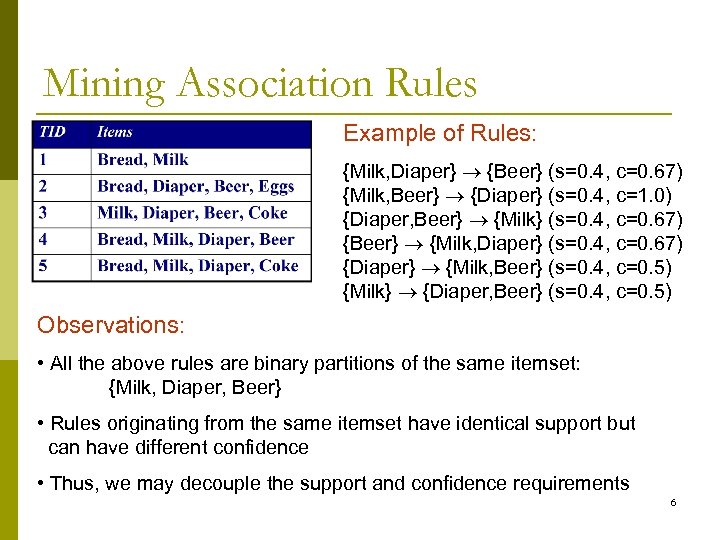
Mining Association Rules Example of Rules: {Milk, Diaper} {Beer} (s=0. 4, c=0. 67) {Milk, Beer} {Diaper} (s=0. 4, c=1. 0) {Diaper, Beer} {Milk} (s=0. 4, c=0. 67) {Beer} {Milk, Diaper} (s=0. 4, c=0. 67) {Diaper} {Milk, Beer} (s=0. 4, c=0. 5) {Milk} {Diaper, Beer} (s=0. 4, c=0. 5) Observations: • All the above rules are binary partitions of the same itemset: {Milk, Diaper, Beer} • Rules originating from the same itemset have identical support but can have different confidence • Thus, we may decouple the support and confidence requirements 6
Mining Association Rules p Two-step approach: 1. Frequent Itemset Generation – 2. Rule Generation – p Generate all itemsets whose support minsup Generate high confidence rules from each frequent itemset, where each rule is a binary partitioning of a frequent itemset Frequent itemset generation is still computationally expensive 7
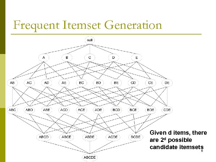
Frequent Itemset Generation Given d items, there are 2 d possible candidate itemsets 8
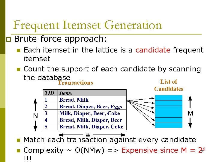
Frequent Itemset Generation p Brute-force approach: n n Each itemset in the lattice is a candidate frequent itemset Count the support of each candidate by scanning the database Match each transaction against every candidate Complexity ~ O(NMw) => Expensive since M = 29 d !!!
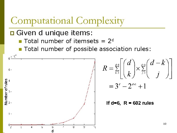
Computational Complexity p Given d unique items: n n Total number of itemsets = 2 d Total number of possible association rules: If d=6, R = 602 rules 10
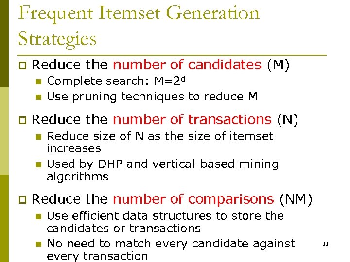
Frequent Itemset Generation Strategies p Reduce the number of candidates (M) n n p Reduce the number of transactions (N) n n p Complete search: M=2 d Use pruning techniques to reduce M Reduce size of N as the size of itemset increases Used by DHP and vertical-based mining algorithms Reduce the number of comparisons (NM) n n Use efficient data structures to store the candidates or transactions No need to match every candidate against every transaction 11
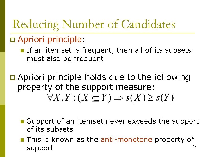
Reducing Number of Candidates p Apriori principle: n p If an itemset is frequent, then all of its subsets must also be frequent Apriori principle holds due to the following property of the support measure: n n Support of an itemset never exceeds the support of its subsets This is known as the anti-monotone property of 12 support
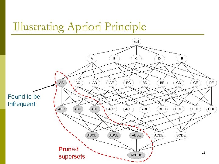
Illustrating Apriori Principle Found to be Infrequent Pruned supersets 13
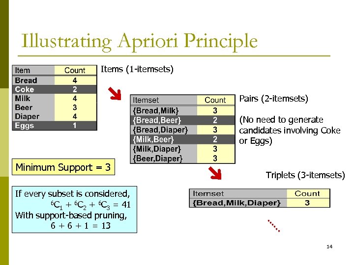
Illustrating Apriori Principle Items (1 -itemsets) Pairs (2 -itemsets) (No need to generate candidates involving Coke or Eggs) Minimum Support = 3 Triplets (3 -itemsets) If every subset is considered, 6 C + 6 C = 41 1 2 3 With support-based pruning, 6 + 1 = 13 14
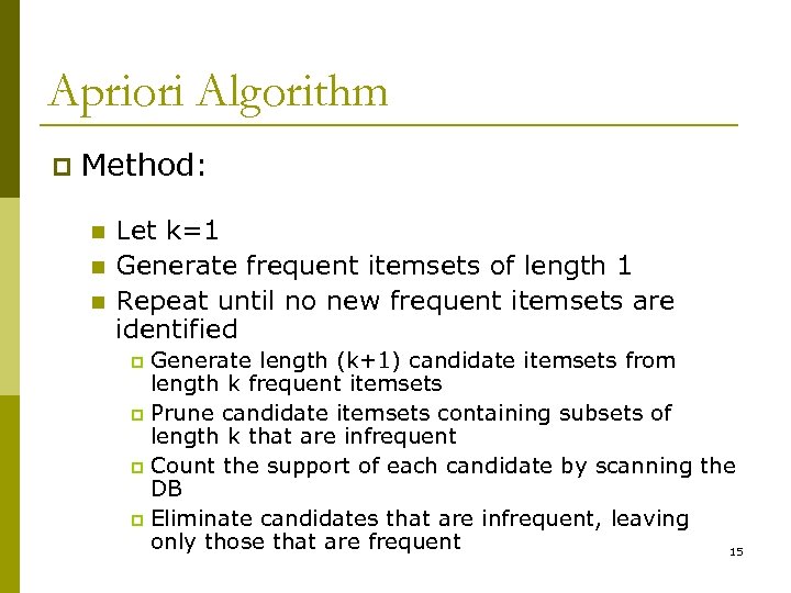
Apriori Algorithm p Method: n n n Let k=1 Generate frequent itemsets of length 1 Repeat until no new frequent itemsets are identified Generate length (k+1) candidate itemsets from length k frequent itemsets p Prune candidate itemsets containing subsets of length k that are infrequent p Count the support of each candidate by scanning the DB p Eliminate candidates that are infrequent, leaving only those that are frequent 15 p
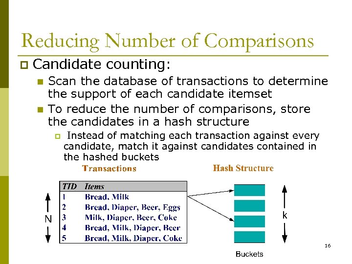
Reducing Number of Comparisons p Candidate counting: n n Scan the database of transactions to determine the support of each candidate itemset To reduce the number of comparisons, store the candidates in a hash structure p Instead of matching each transaction against every candidate, match it against candidates contained in the hashed buckets 16
Review What are the association rules? p What are the frequent itemsets? p What are support/supporting count? p What’s apriori principle? p How to mine FIM? p 17
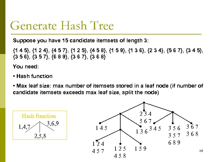
Generate Hash Tree Suppose you have 15 candidate itemsets of length 3: {1 4 5}, {1 2 4}, {4 5 7}, {1 2 5}, {4 5 8}, {1 5 9}, {1 3 6}, {2 3 4}, {5 6 7}, {3 4 5}, {3 5 6}, {3 5 7}, {6 8 9}, {3 6 7}, {3 6 8} You need: • Hash function • Max leaf size: max number of itemsets stored in a leaf node (if number of candidate itemsets exceeds max leaf size, split the node) Hash function 3, 6, 9 1, 4, 7 234 567 345 136 145 2, 5, 8 124 457 125 458 159 356 357 689 367 368 18
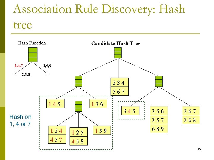
Association Rule Discovery: Hash tree Hash Function 1, 4, 7 Candidate Hash Tree 3, 6, 9 2, 5, 8 234 567 145 136 345 Hash on 1, 4 or 7 124 125 457 356 357 689 367 368 458 159 19
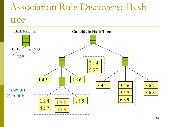
Association Rule Discovery: Hash tree Hash Function 1, 4, 7 Candidate Hash Tree 3, 6, 9 2, 5, 8 234 567 145 136 345 Hash on 2, 5 or 8 124 125 457 356 357 689 367 368 458 159 20
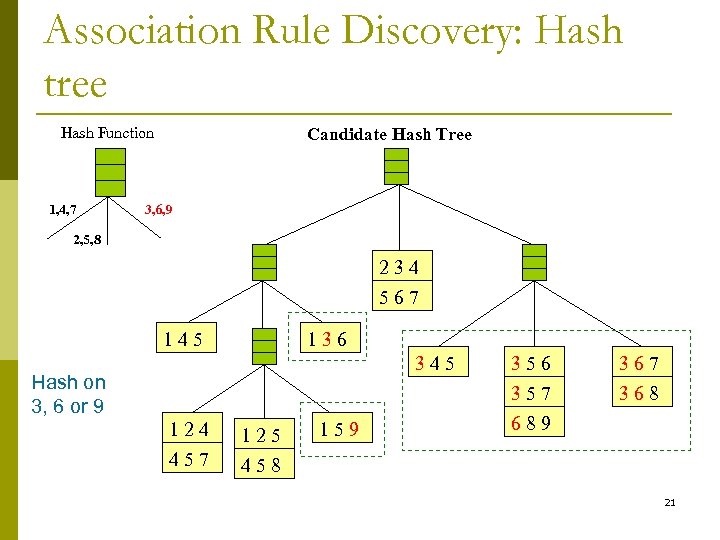
Association Rule Discovery: Hash tree Hash Function 1, 4, 7 Candidate Hash Tree 3, 6, 9 2, 5, 8 234 567 145 136 345 Hash on 3, 6 or 9 124 125 457 356 357 689 367 368 458 159 21
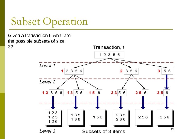
Subset Operation Given a transaction t, what are the possible subsets of size 3? 22
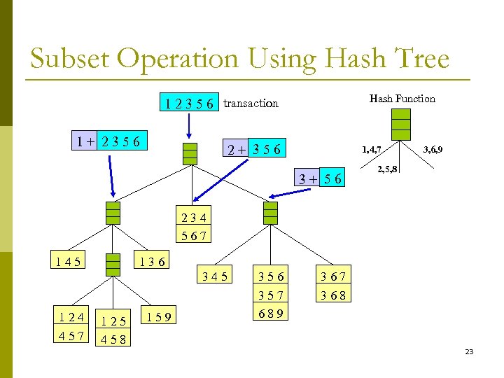
Subset Operation Using Hash Tree Hash Function 1 2 3 5 6 transaction 1+ 2356 2+ 356 1, 4, 7 3+ 56 3, 6, 9 2, 5, 8 234 567 145 136 345 124 457 125 458 159 356 357 689 367 368 23
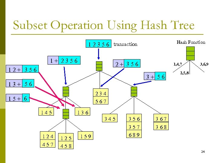
Subset Operation Using Hash Tree Hash Function 1 2 3 5 6 transaction 1+ 2356 2+ 356 1, 4, 7 3+ 56 3, 6, 9 2, 5, 8 13+ 56 234 567 15+ 6 145 136 345 124 457 125 458 159 356 357 689 367 368 24
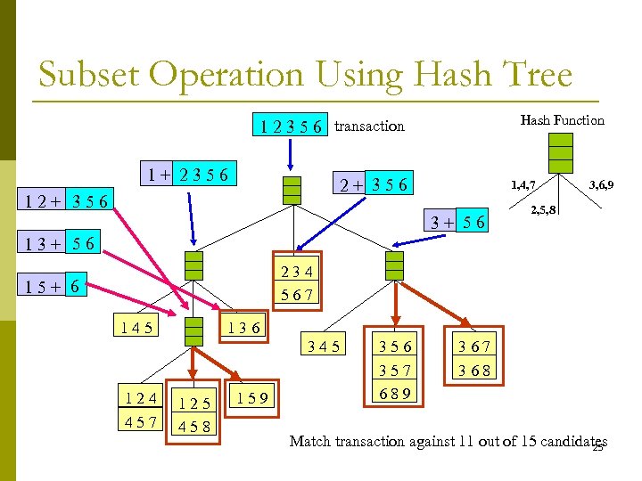
Subset Operation Using Hash Tree Hash Function 1 2 3 5 6 transaction 1+ 2356 2+ 356 1, 4, 7 3+ 56 3, 6, 9 2, 5, 8 13+ 56 234 567 15+ 6 145 136 345 124 457 125 458 159 356 357 689 367 368 Match transaction against 11 out of 15 candidates 25
How to Generate Candidates? p Suppose the items in Lk-1 are listed in an order p Step 1: self-joining Lk-1 insert into Ck select p. item 1, p. item 2, …, p. itemk-1, q. itemk-1 from Lk-1 p, Lk-1 q where p. item 1=q. item 1, …, p. itemk-2=q. itemk-2, p. itemk-1 < q. itemk-1 p Step 2: pruning forall itemsets c in Ck do forall (k-1)-subsets s of c do if (s is not in Lk-1) then delete c from Ck 26
Challenges of Frequent Pattern Mining p Challenges n n Huge number of candidates n p Multiple scans of transaction database Tedious workload of support counting for candidates Improving Apriori: general ideas n Reduce passes of transaction database scans n Shrink number of candidates n Facilitate support counting of candidates 27
Partition: Scan Database Only Twice p Any itemset that is potentially frequent in DB must be frequent in at least one of the partitions of DB n Scan 1: partition database and find local frequent patterns n p Scan 2: consolidate global frequent patterns A. Savasere, E. Omiecinski, and S. Navathe. An efficient algorithm for mining association in large databases. In VLDB’ 95 28
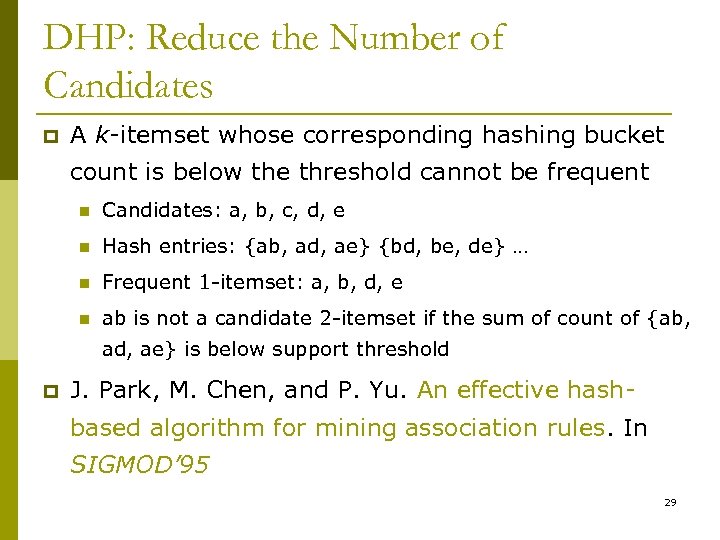
DHP: Reduce the Number of Candidates p A k-itemset whose corresponding hashing bucket count is below the threshold cannot be frequent n Candidates: a, b, c, d, e n Hash entries: {ab, ad, ae} {bd, be, de} … n Frequent 1 -itemset: a, b, d, e n ab is not a candidate 2 -itemset if the sum of count of {ab, ad, ae} is below support threshold p J. Park, M. Chen, and P. Yu. An effective hashbased algorithm for mining association rules. In SIGMOD’ 95 29
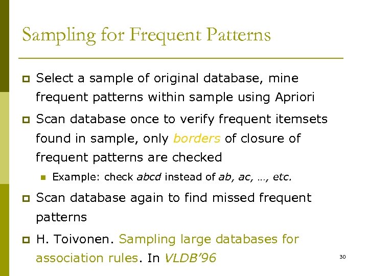
Sampling for Frequent Patterns p Select a sample of original database, mine frequent patterns within sample using Apriori p Scan database once to verify frequent itemsets found in sample, only borders of closure of frequent patterns are checked n p Example: check abcd instead of ab, ac, …, etc. Scan database again to find missed frequent patterns p H. Toivonen. Sampling large databases for association rules. In VLDB’ 96 30
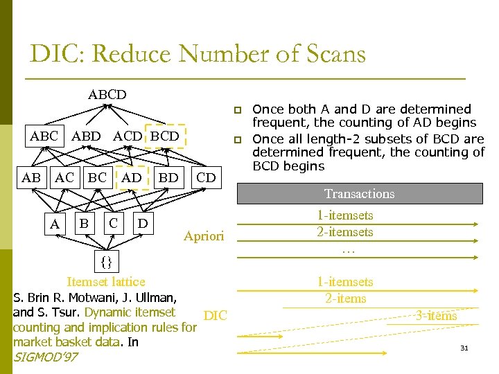
DIC: Reduce Number of Scans ABCD p ABC ABD ACD BCD AB AC BC AD BD p CD Once both A and D are determined frequent, the counting of AD begins Once all length-2 subsets of BCD are determined frequent, the counting of BCD begins Transactions B A C D Apriori {} Itemset lattice S. Brin R. Motwani, J. Ullman, and S. Tsur. Dynamic itemset DIC counting and implication rules for market basket data. In SIGMOD’ 97 1 -itemsets 2 -itemsets … 1 -itemsets 2 -items 31
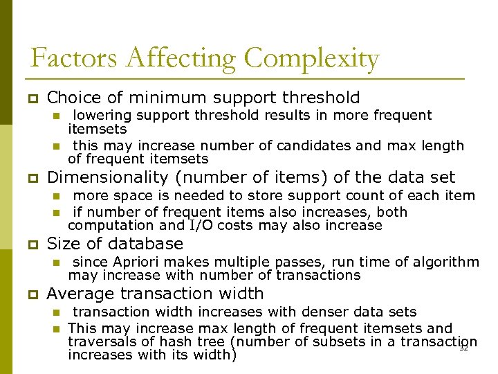
Factors Affecting Complexity p Choice of minimum support threshold n n p Dimensionality (number of items) of the data set n n p more space is needed to store support count of each item if number of frequent items also increases, both computation and I/O costs may also increase Size of database n p lowering support threshold results in more frequent itemsets this may increase number of candidates and max length of frequent itemsets since Apriori makes multiple passes, run time of algorithm may increase with number of transactions Average transaction width n n transaction width increases with denser data sets This may increase max length of frequent itemsets and traversals of hash tree (number of subsets in a transaction 32 increases with its width)
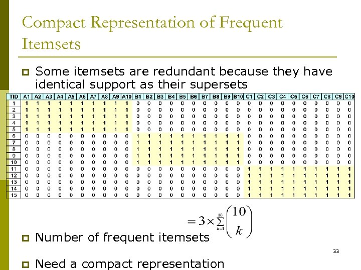
Compact Representation of Frequent Itemsets p Some itemsets are redundant because they have identical support as their supersets p Number of frequent itemsets 33 p Need a compact representation
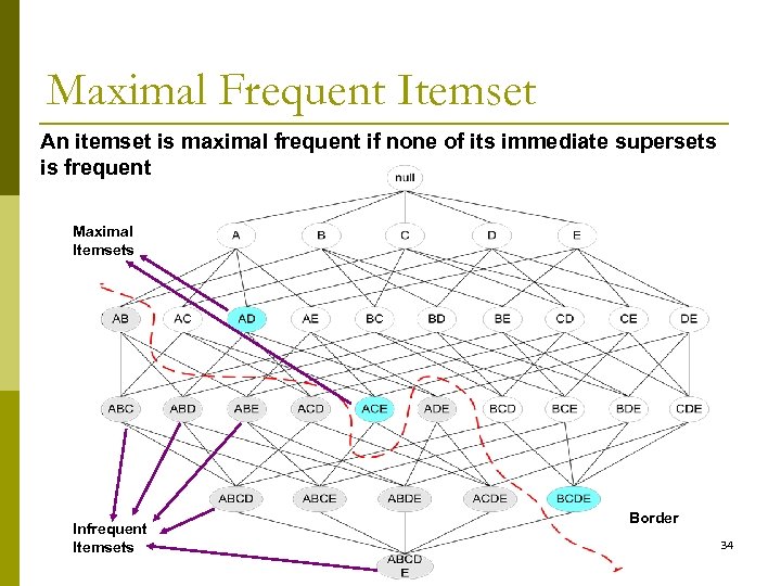
Maximal Frequent Itemset An itemset is maximal frequent if none of its immediate supersets is frequent Maximal Itemsets Infrequent Itemsets Border 34
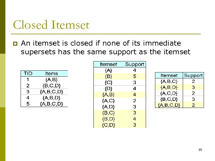
Closed Itemset p An itemset is closed if none of its immediate supersets has the same support as the itemset 35
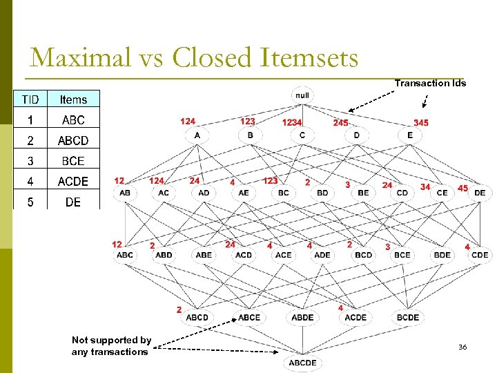
Maximal vs Closed Itemsets Transaction Ids Not supported by any transactions 36
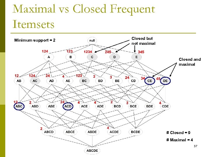
Maximal vs Closed Frequent Itemsets Minimum support = 2 Closed but not maximal Closed and maximal # Closed = 9 # Maximal = 4 37
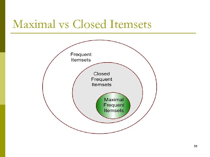
Maximal vs Closed Itemsets 38
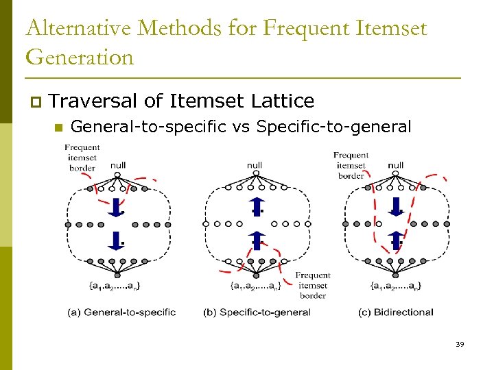
Alternative Methods for Frequent Itemset Generation p Traversal of Itemset Lattice n General-to-specific vs Specific-to-general 39
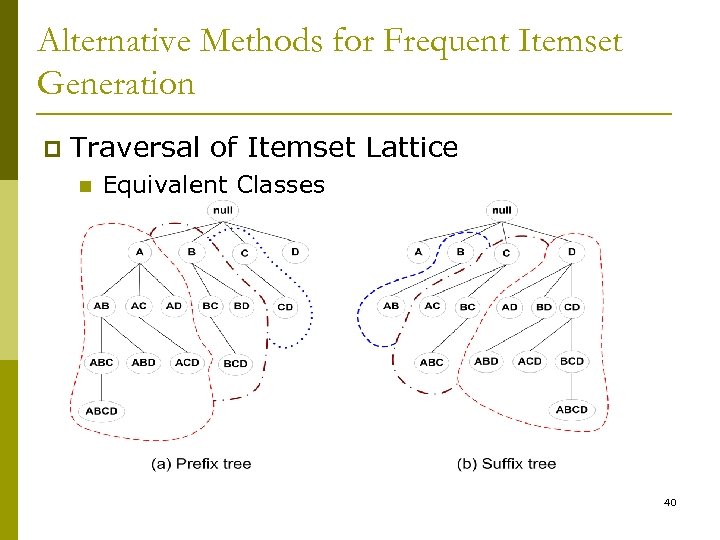
Alternative Methods for Frequent Itemset Generation p Traversal of Itemset Lattice n Equivalent Classes 40
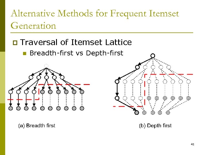
Alternative Methods for Frequent Itemset Generation p Traversal of Itemset Lattice n Breadth-first vs Depth-first 41
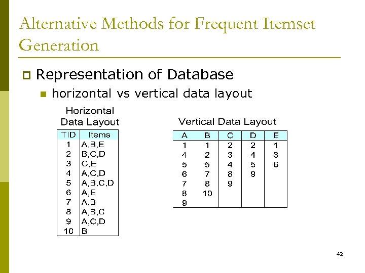
Alternative Methods for Frequent Itemset Generation p Representation of Database n horizontal vs vertical data layout 42
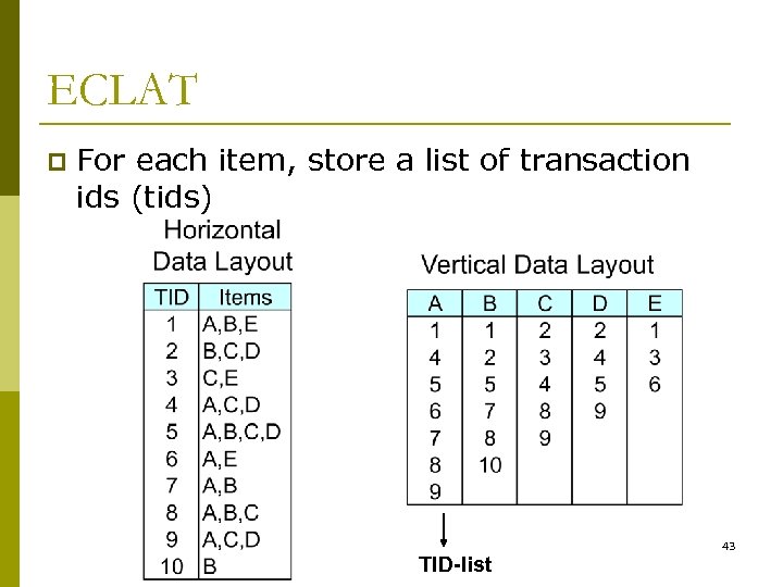
ECLAT p For each item, store a list of transaction ids (tids) TID-list 43
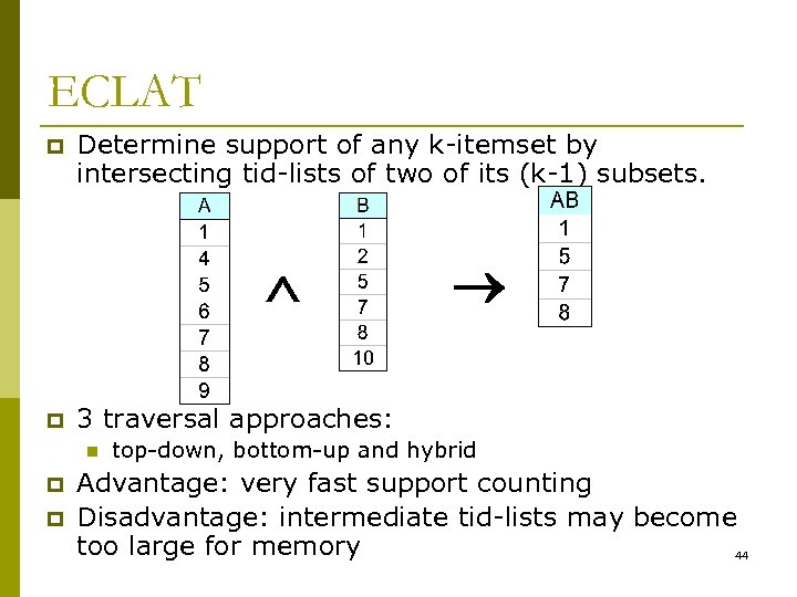
ECLAT p Determine support of any k-itemset by intersecting tid-lists of two of its (k-1) subsets. p 3 traversal approaches: n p p top-down, bottom-up and hybrid Advantage: very fast support counting Disadvantage: intermediate tid-lists may become too large for memory 44
FP-growth Algorithm p Use a compressed representation of the database using an FP-tree p Once an FP-tree has been constructed, it uses a recursive divide-and-conquer approach to mine the frequent itemsets 45
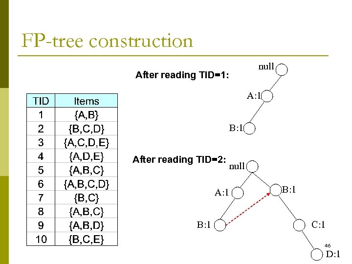
FP-tree construction null After reading TID=1: A: 1 B: 1 After reading TID=2: A: 1 B: 1 null B: 1 C: 1 46 D: 1
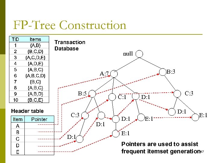
FP-Tree Construction Transaction Database null B: 3 A: 7 B: 5 Header table C: 1 C: 3 D: 1 D: 1 E: 1 Pointers are used to assist frequent itemset generation 47
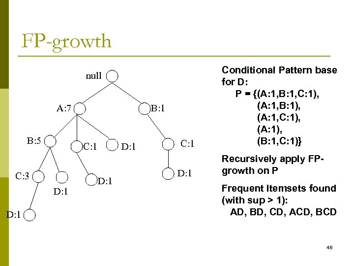
FP-growth C: 1 Conditional Pattern base for D: P = {(A: 1, B: 1, C: 1), (A: 1, B: 1), (A: 1, C: 1), (A: 1), (B: 1, C: 1)} D: 1 Recursively apply FPgrowth on P null A: 7 B: 5 C: 1 C: 3 D: 1 B: 1 D: 1 Frequent Itemsets found (with sup > 1): AD, BD, CD, ACD, BCD 48
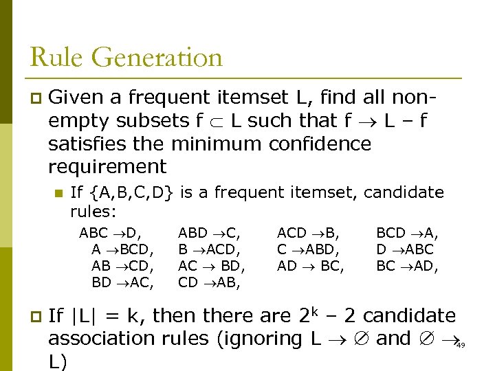
Rule Generation p Given a frequent itemset L, find all nonempty subsets f L such that f L – f satisfies the minimum confidence requirement n If {A, B, C, D} is a frequent itemset, candidate rules: ABC D, A BCD, AB CD, BD AC, p ABD C, B ACD, AC BD, CD AB, ACD B, C ABD, AD BC, BCD A, D ABC BC AD, If |L| = k, then there are 2 k – 2 candidate association rules (ignoring L and L) 49
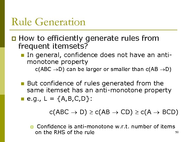
Rule Generation p How to efficiently generate rules from frequent itemsets? n In general, confidence does not have an antimonotone property c(ABC D) can be larger or smaller than c(AB D) n n But confidence of rules generated from the same itemset has an anti-monotone property e. g. , L = {A, B, C, D}: c(ABC D) c(AB CD) c(A BCD) p Confidence is anti-monotone w. r. t. number of items 50 on the RHS of the rule
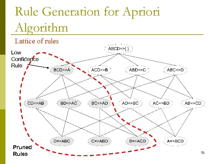
Rule Generation for Apriori Algorithm Lattice of rules Low Confidence Rule Pruned Rules 51
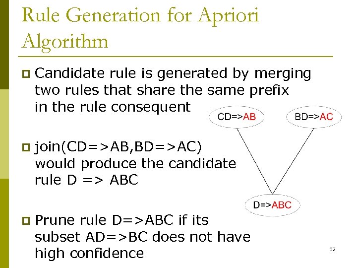
Rule Generation for Apriori Algorithm p Candidate rule is generated by merging two rules that share the same prefix in the rule consequent p join(CD=>AB, BD=>AC) would produce the candidate rule D => ABC p Prune rule D=>ABC if its subset AD=>BC does not have high confidence 52
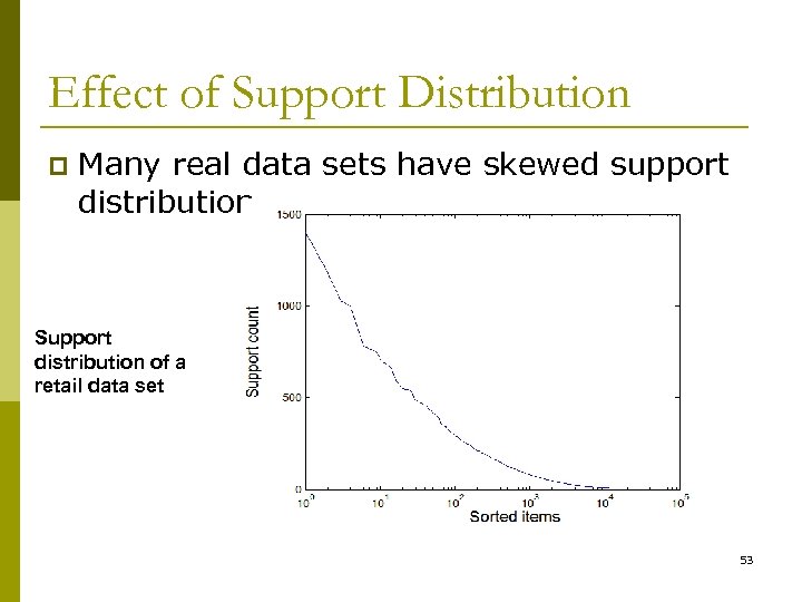
Effect of Support Distribution p Many real data sets have skewed support distribution Support distribution of a retail data set 53
Effect of Support Distribution p How to set the appropriate minsup threshold? n n p If minsup is set too high, we could miss itemsets involving interesting rare items (e. g. , expensive products) If minsup is set too low, it is computationally expensive and the number of itemsets is very large Using a single minimum support threshold may not be effective 54
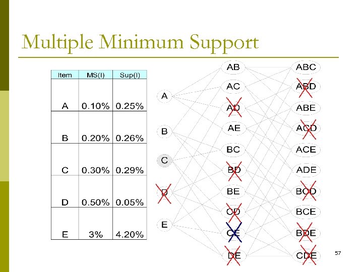
Multiple Minimum Support p How to apply multiple minimum supports? n n MS(i): minimum support for item i e. g. : MS(Milk)=5%, MS(Coke) = 3%, MS(Broccoli)=0. 1%, MS(Salmon)=0. 5% MS({Milk, Broccoli}) = min (MS(Milk), MS(Broccoli)) = 0. 1% Challenge: Support is no longer anti-monotone Suppose: Support(Milk, Coke) = 1. 5% and Support(Milk, Coke, Broccoli) = 0. 5% p {Milk, Coke} is infrequent but {Milk, Coke, Broccoli} is 55 frequent p
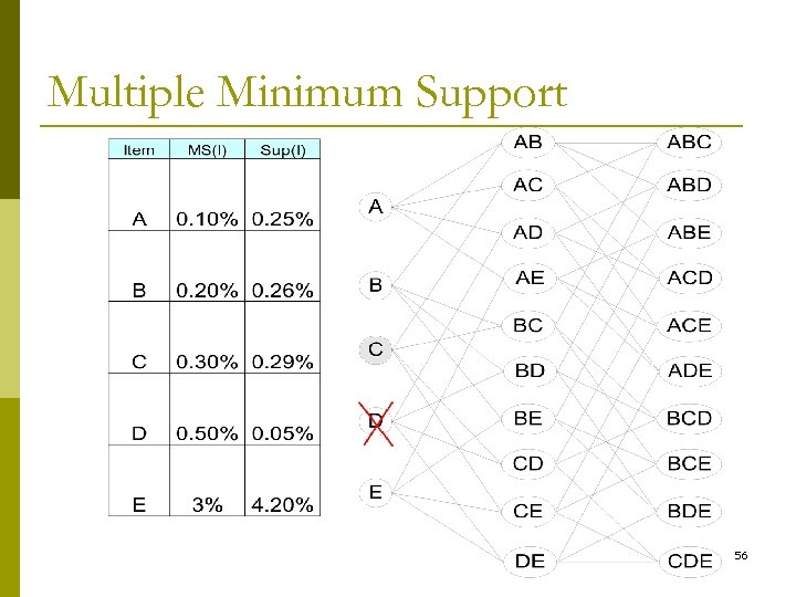
Multiple Minimum Support 56
Multiple Minimum Support 57
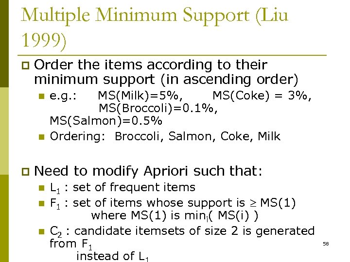
Multiple Minimum Support (Liu 1999) p Order the items according to their minimum support (in ascending order) n n p e. g. : MS(Milk)=5%, MS(Coke) = 3%, MS(Broccoli)=0. 1%, MS(Salmon)=0. 5% Ordering: Broccoli, Salmon, Coke, Milk Need to modify Apriori such that: n n n L 1 : set of frequent items F 1 : set of items whose support is MS(1) where MS(1) is mini( MS(i) ) C 2 : candidate itemsets of size 2 is generated from F 1 instead of L 58
Multiple Minimum Support (Liu 1999) p Modifications to Apriori: n In traditional Apriori, A candidate (k+1)-itemset is generated by merging two frequent itemsets of size k p The candidate is pruned if it contains any infrequent subsets of size k p n Pruning step has to be modified: Prune only if subset contains the first item p e. g. : Candidate={Broccoli, Coke, Milk} (ordered according to minimum support) p {Broccoli, Coke} and {Broccoli, Milk} are frequent but {Coke, Milk} is infrequent p § Candidate is not pruned because {Coke, Milk} does not 59 contain the first item, i. e. , Broccoli.
Mining Various Kinds of Association Rules p Mining multilevel association p Miming multidimensional association p Mining quantitative association p Mining interesting correlation patterns 60
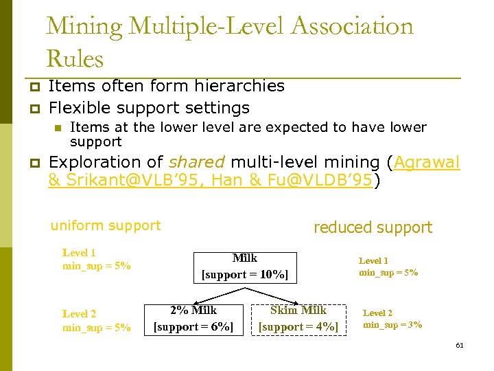
Mining Multiple-Level Association Rules p p Items often form hierarchies Flexible support settings n p Items at the lower level are expected to have lower support Exploration of shared multi-level mining (Agrawal & Srikant@VLB’ 95, Han & Fu@VLDB’ 95) uniform support Level 1 min_sup = 5% Level 2 min_sup = 5% reduced support Milk [support = 10%] 2% Milk [support = 6%] Skim Milk [support = 4%] Level 1 min_sup = 5% Level 2 min_sup = 3% 61
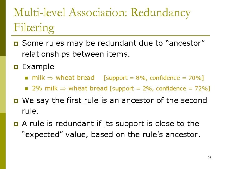
Multi-level Association: Redundancy Filtering p Some rules may be redundant due to “ancestor” relationships between items. p Example n milk wheat bread n 2% milk wheat bread [support = 2%, confidence = 72%] [support = 8%, confidence = 70%] p We say the first rule is an ancestor of the second rule. p A rule is redundant if its support is close to the “expected” value, based on the rule’s ancestor. 62
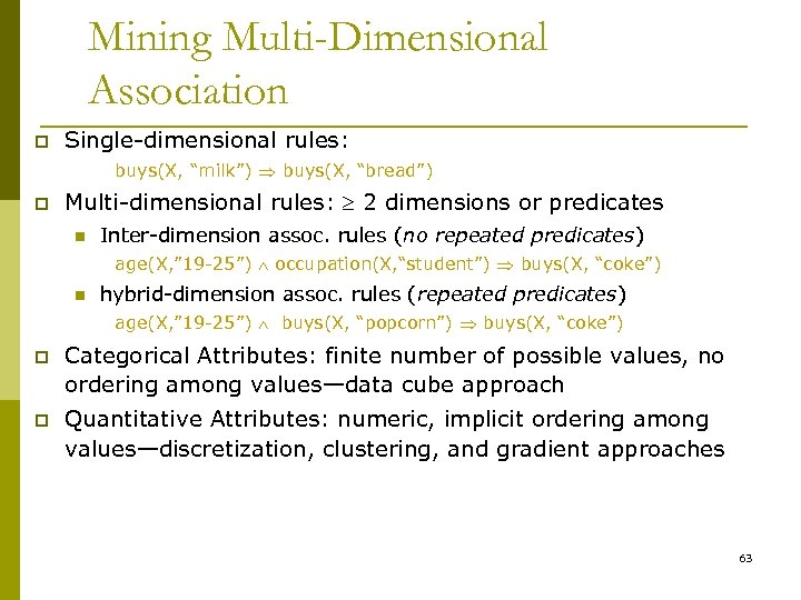
Mining Multi-Dimensional Association p Single-dimensional rules: buys(X, “milk”) buys(X, “bread”) p Multi-dimensional rules: 2 dimensions or predicates n Inter-dimension assoc. rules (no repeated predicates) age(X, ” 19 -25”) occupation(X, “student”) buys(X, “coke”) n hybrid-dimension assoc. rules (repeated predicates) age(X, ” 19 -25”) buys(X, “popcorn”) buys(X, “coke”) p Categorical Attributes: finite number of possible values, no ordering among values—data cube approach p Quantitative Attributes: numeric, implicit ordering among values—discretization, clustering, and gradient approaches 63
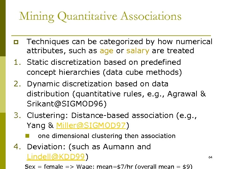
Mining Quantitative Associations p Techniques can be categorized by how numerical attributes, such as age or salary are treated 1. Static discretization based on predefined concept hierarchies (data cube methods) 2. Dynamic discretization based on data distribution (quantitative rules, e. g. , Agrawal & Srikant@SIGMOD 96) 3. Clustering: Distance-based association (e. g. , Yang & Miller@SIGMOD 97) n one dimensional clustering then association 4. Deviation: (such as Aumann and Lindell@KDD 99) Sex = female => Wage: mean=$7/hr (overall mean = $9) 64
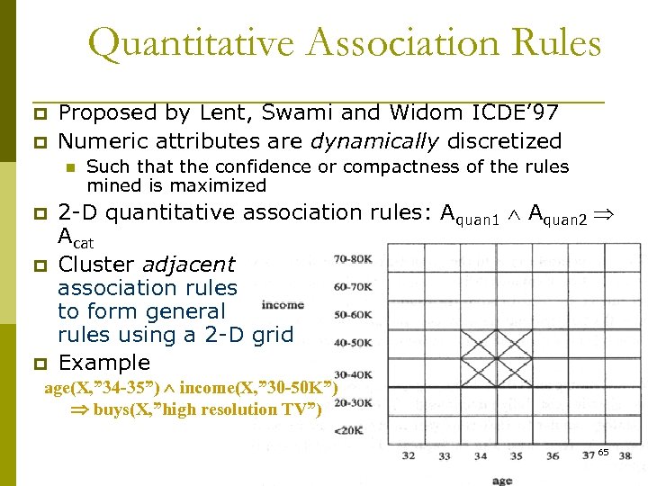
Quantitative Association Rules p p Proposed by Lent, Swami and Widom ICDE’ 97 Numeric attributes are dynamically discretized n p p p Such that the confidence or compactness of the rules mined is maximized 2 -D quantitative association rules: Aquan 1 Aquan 2 Acat Cluster adjacent association rules to form general rules using a 2 -D grid Example age(X, ” 34 -35”) income(X, ” 30 -50 K”) buys(X, ”high resolution TV”) 65
Mining Other Interesting Patterns p Flexible support constraints (Wang et al. @ VLDB’ 02) n n p Some items (e. g. , diamond) may occur rarely but are valuable Customized supmin specification and application Top-K closed frequent patterns (Han, et al. @ ICDM’ 02) n Hard to specify supmin, but top-k with lengthmin is more desirable n Dynamically raise supmin in FP-tree construction and mining, and select most promising path to mine 66
Pattern Evaluation p Association rule algorithms tend to produce too many rules n n many of them are uninteresting or redundant Redundant if {A, B, C} {D} and {A, B} {D} have same support & confidence p Interestingness measures can be used to prune/rank the derived patterns p In the original formulation of association rules, support & confidence are the only measures used 67
![Interestingness Measure: Correlations (Lift) p play basketball eat cereal [40%, 66. 7%] is misleading Interestingness Measure: Correlations (Lift) p play basketball eat cereal [40%, 66. 7%] is misleading](https://present5.com/presentation/6d1749c2eedc1b9056679efb698c4f64/image-68.jpg)
Interestingness Measure: Correlations (Lift) p play basketball eat cereal [40%, 66. 7%] is misleading n p The overall % of students eating cereal is 75% > 66. 7%. play basketball not eat cereal [20%, 33. 3%] is more accurate, although with lower support and confidence p Measure of dependent/correlated events: lift Basketb all Not basketball Sum (row) Cereal 2000 1750 3750 Not cereal 1000 250 1250 Sum(col. ) 3000 2000 5000 68
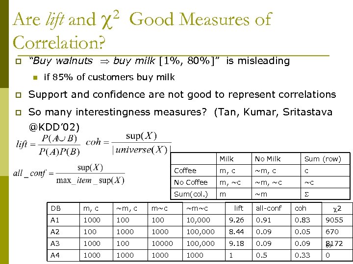
Are lift and 2 Good Measures of Correlation? p “Buy walnuts buy milk [1%, 80%]” is misleading n if 85% of customers buy milk p Support and confidence are not good to represent correlations p So many interestingness measures? (Tan, Kumar, Sritastava @KDD’ 02) Milk No Milk Sum (row) Coffee m, c ~m, c c No Coffee m, ~c ~c Sum(col. ) m ~m DB m, c ~m, c m~c ~m~c A 1 1000 100 10, 000 A 2 1000 A 3 1000 100 A 4 1000 lift 2 all-conf coh 9. 26 0. 91 0. 83 9055 100, 000 8. 44 0. 09 0. 05 670 10000 100, 000 9. 18 0. 09 8172 69 1000 1 0. 5 0. 33 0
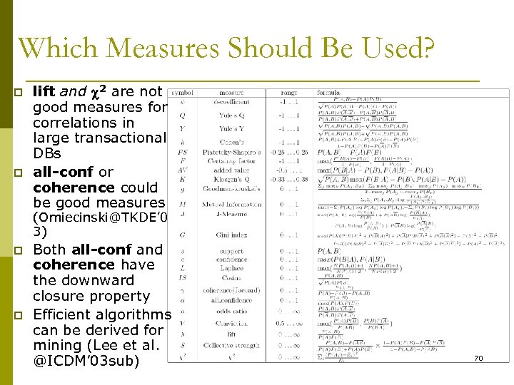
Which Measures Should Be Used? p p lift and 2 are not good measures for correlations in large transactional DBs all-conf or coherence could be good measures (Omiecinski@TKDE’ 0 3) p p Both all-conf and coherence have the downward closure property Efficient algorithms can be derived for mining (Lee et al. @ICDM’ 03 sub) 70
6d1749c2eedc1b9056679efb698c4f64.ppt