c8311e1487ce7bcb7d7fb886f6863980.ppt
- Количество слайдов: 17
 Assessing Predictors of Software Defects Tim Menzies Justin S. Di Stefano Andres Orrego Robert (Mike) Chapman tim@menzies. us justin@lostportal. net andres. s. orrego@ivv. nasa. gov robert. m. chapman@ivv. nasa. gov Workshop on Predictive Software Models (PSM 2004) September 17, 2004 Palmer House Hilton Hotel Chicago, IL, USA http: // menzies. us/pdf/04 psm. pdf 1
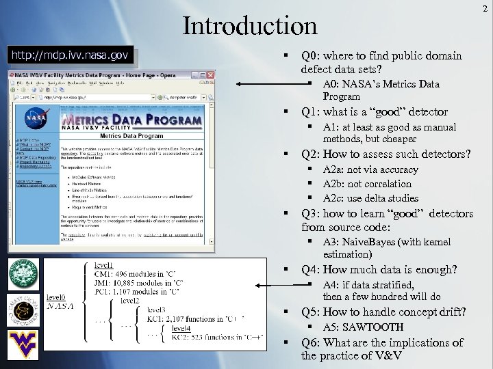 Introduction http: //mdp. ivv. nasa. gov § Q 0: where to find public domain defect data sets? § A 0: NASA’s Metrics Data Program § Q 1: what is a “good” detector § A 1: at least as good as manual methods, but cheaper § Q 2: How to assess such detectors? § A 2 a: not via accuracy § A 2 b: not correlation § A 2 c: use delta studies § Q 3: how to learn “good” detectors from source code: § A 3: Naive. Bayes (with kernel estimation) § Q 4: How much data is enough? § A 4: if data stratified, then a few hundred will do § Q 5: How to handle concept drift? § A 5: SAWTOOTH § Q 6: What are the implications of the practice of V&V 2
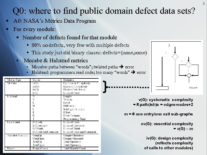 Q 0: where to find public domain defect data sets? § A 0: NASA’s Metrics Data Program § For every module: § Number of defects found for that module § 80% no defects, very few with multiple defects § This study just did binary classes: defects={none, some) § Mccabe & Halstead metrics • Mccabe: paths between “words”; twisted paths error • Halstead: programmers read code; too many “words” error v(G): cyclomatic complexity = # path(ish)s = edges-nodes+2 m = # one entry/one exit sub-graphs ev(G): essential complexity = v(G) – m iv(G): design complexity (reflects complexity of calls to other modules) 3
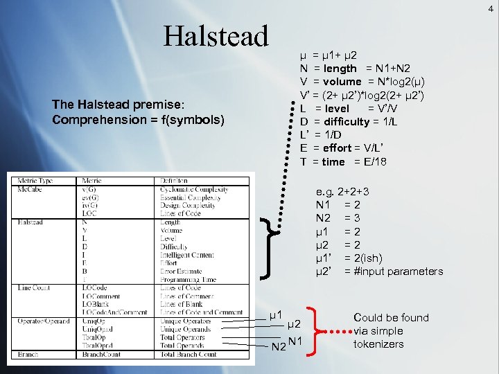 4 Halstead µ = µ 1+ µ 2 N = length = N 1+N 2 V = volume = N*log 2(µ) V’ = (2+ µ 2’)*log 2(2+ µ 2’) L = level = V’/V D = difficulty = 1/L L’ = 1/D E = effort = V/L’ T = time = E/18 The Halstead premise: Comprehension = f(symbols) e. g. 2+2+3 N 1 = 2 N 2 = 3 µ 1 = 2 µ 2 = 2 µ 1’ = 2(ish) µ 2’ = #input parameters µ 1 N 2 µ 2 N 1 Could be found via simple tokenizers
 5 By the way… § Halstead and Mccabe have bad press § Sheppard & Ince, Fenton, Glass, etc… § Our reply: § Ideally, want better feature extractors from code § Halstead/Mccabe are decades old § ? ? use Polyspace or Code. Surfer to define better measures. § Model-based comprehension is better but… § Sometimes, these code measures is all you can get: § IV&V § Audits of code developed off-shore § Anyway, we can achieve human-level competency at defection, § using less effort § ? ? first such report in the literature § And our results are repeatable, refutable § Based on public domain data sets
 6 Question 1: what is a “good” defect detector? § Answer: at least as good as manual methods, but cheaper § Effort: § Local IV&V method: § 8 LOC/minute § Schull “structured reading”: § Per 500 LOC, 2 hours to prepare, 2 hours to inspect § Probability of detection (PD) } } Not widely accepted Our goal: 40%. . 60%
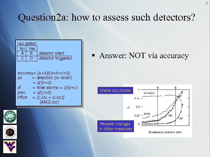 7 Question 2 a: how to assess such detectors? has defect No Yes A B detector silent C D detector triggered accuracy= (a+d)/(a+b+c+d) pd = detection (or recall) = d/(b+d) pf = false alarms = c/(a+c) prec = d/(c+d) Effort = (C. loc + D. loc)/ (ABCD. loc) § Answer: NOT via accuracy Stable accuracies Massive changes in other measures
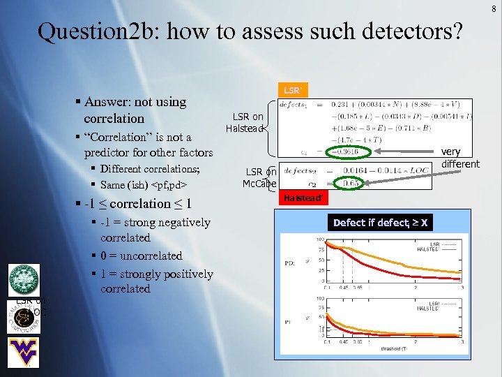 8 Question 2 b: how to assess such detectors? § Answer: not using correlation § “Correlation” is not a predictor for other factors § Different correlations; § Same (ish)
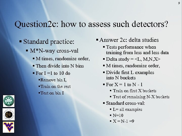 9 Question 2 c: how to assess such detectors? § Standard practice: § M*N-way cross-val § M times, randomize order, § Then divide into N bins § For I =1 to 10 do §Remove bin I, §Train on the rest §Test on bin I § Answer 2 c: delta studies § Tests performance when training from less and less data § Delta study =
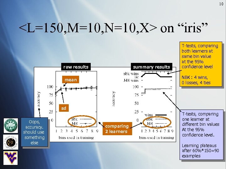 10
10
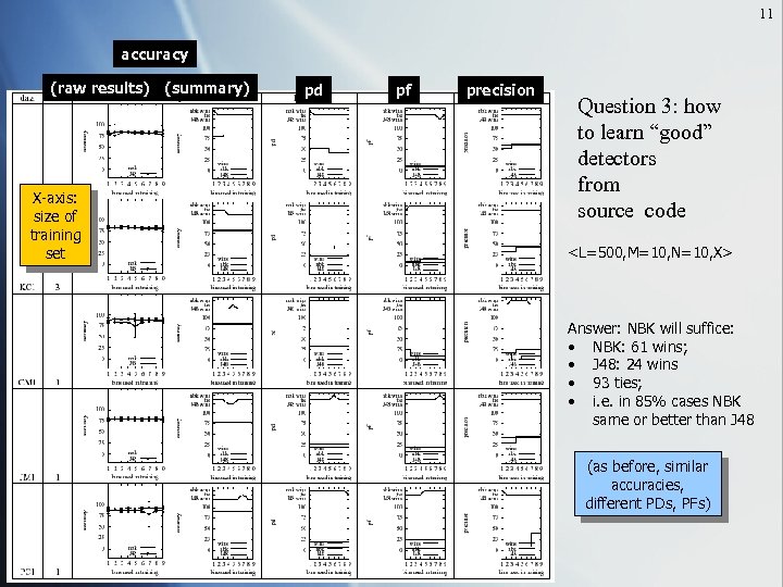 11 accuracy (raw results) (summary) X-axis: size of training set pd pf precision Question 3: how to learn “good” detectors from source code
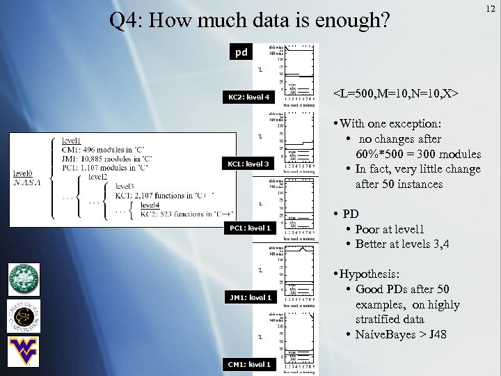 Q 4: How much data is enough? pd KC 2: level 4 KC 1: level 3 PC 1: level 1 JM 1: level 1 CM 1: level 1
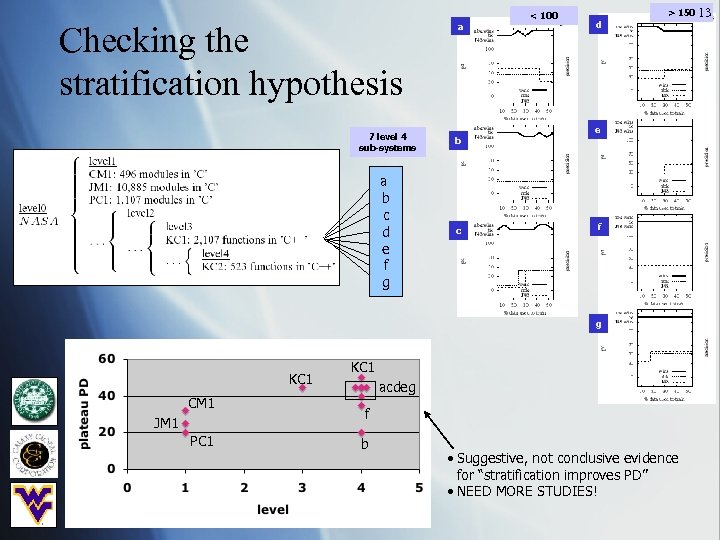 Checking the stratification hypothesis a < 100 d > 150 13 e 7 level 4 sub-systems b a b c d e f g c f g KC 1 CM 1 JM 1 PC 1 KC 1 acdeg f b • Suggestive, not conclusive evidence for “stratification improves PD” • NEED MORE STUDIES!
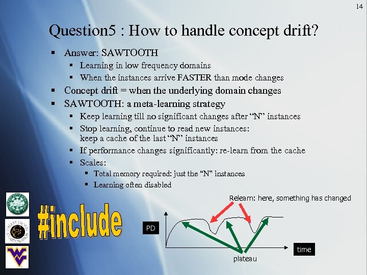 14 Question 5 : How to handle concept drift? § Answer: SAWTOOTH § Learning in low frequency domains § When the instances arrive FASTER than mode changes § Concept drift = when the underlying domain changes § SAWTOOTH: a meta-learning strategy § Keep learning till no significant changes after “N” instances § Stop learning, continue to read new instances: keep a cache of the last “N” instances § If performance changes significantly: re-learn from the cache § Scales: § Total memory required: just the “N” instances § Learning often disabled Relearn: here, something has changed PD time plateau
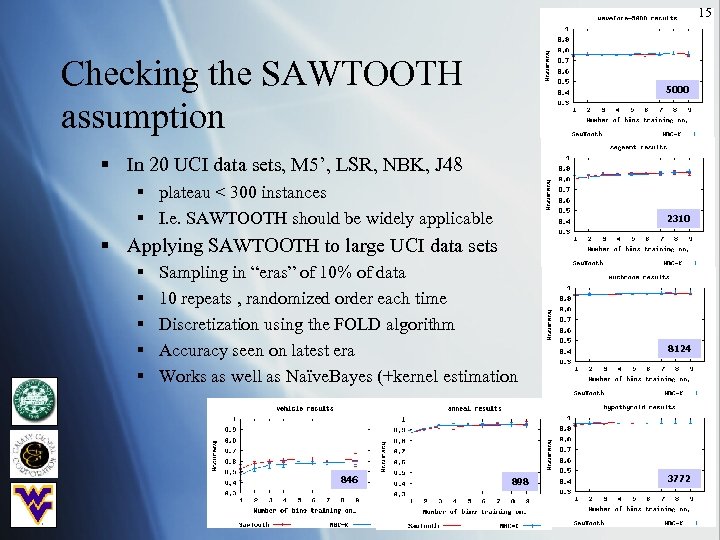 15 Checking the SAWTOOTH assumption 5000 § In 20 UCI data sets, M 5’, LSR, NBK, J 48 § plateau < 300 instances § I. e. SAWTOOTH should be widely applicable 2310 § Applying SAWTOOTH to large UCI data sets § § § Sampling in “eras” of 10% of data 10 repeats , randomized order each time Discretization using the FOLD algorithm Accuracy seen on latest era Works as well as Naïve. Bayes (+kernel estimation 846 898 8124 3772
 16 Q 6: What are the implications for the practice of V&V? § Defect detectors based on static code measures § Can compete with manual code inspections § Requires far less effort § When working on a new sub-system § Do inspection of the first 50 modules § Only inspect the modules selected by the detector
 17 Conclusions (notes for researchers) § § Do repeatable experiments on public domain data. Compare results to known baselines in the SE literature Assess using delta studies Don’t select detectors based on accuracy/correlation § may not predict for PD/PF § Check for: § Plateaus after < 100 examples § Stratification increasing PDs


