aea5062d91041b32cf2fff2bd3fac67e.ppt
- Количество слайдов: 45

Assesing Store Performance Equitably Gábor Pauler, Ph. D. Associated Professor Depatment of Computer Science Faculty of Engineering University of Pécs, Hungary Phone: +36 -309 -015 -488, E-mail: gjpauler@acsu. buffalo. edu Minaksi Trivedi, Ph. D. Associated Professor, Department of Marketing Jacobs School of Management SUNY at Buffalo, NY, USA Phone: +1(716)645 -3214 E-mail: mtrivedi@acsu. buffalo. edu Presented at PTE-TTK Oct 27, 2010 Dinesh K. Gauri, Ph. D. -student Department of Marketing Jacobs School of Management SUNY at Buffalo, NY, USA Phone: +1(716)645 -3331 E-mail: dkgauri@acsu. buffalo. edu
Content of the Presentation Significance of benchmarking stores Literature overview Infinite trading are approach: the original Huff-model Finite trading area approaches Radial Polygonal Cubic splines Gradual approaches Our store benchmarking model: Basic assumptions Objectives Input data Geocoding of stores, distance computations Analyzing satelite photos Basic equations of the model Estimation of parameters Testing of parameter estimation Benchmarking measures Practical application Evaluating estimated parameters Spatial mapping of the results Summary, References
Paradigms of Supermarket Chain Management Discount-Orientated Database. Marketing Orientated The purpose of Loyalty Cards do not is to generate loyalty Give out rewards to generate Give out rewards to collect store traffic and sales customer info, identify high valued customers Selective promotion of high Mass-promotion programs valued costumers accessible for everybody Profit-driven Volume-driven Benchmarking: multi. Benchmarking: only the layered (stores, regions, whole chain to competitors, segments) Database: OLAP Database: Relational Examples: Tesco, UK 1998 14 M Cards Safeway, UK 1998, 10 M Sainsbury, UK 1999 13 M Cards, fails in 2000, $42 M Cards lost ASDA, UK 1999, 360 K Cards, Success in fierce competition for demanding customers back to EDLP
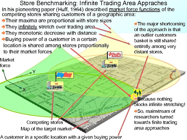
Store Benchmarking: Infinite Trading Area Appraches In his pioneering paper (Huff, 1964) described market force functions of the competing stores sharing customers of a geographic area: Their maxima are proportional with store sizes The major shortcoming They infinitely stretch over trading area of the approach is that They monotonic decrease with distance an outlier customers Buying power of a customer in a certain basket is still shared location is shared among stores proportionally entirelly among very distant stores, to their market forces Po. Ps Market force Y Big. Buy X Competing stores Map of the target market A customer in a specific location with a given buying power $ Because nothing blocks infinite stretching! So, mainstream of researchers turned towards finite trading area approaches
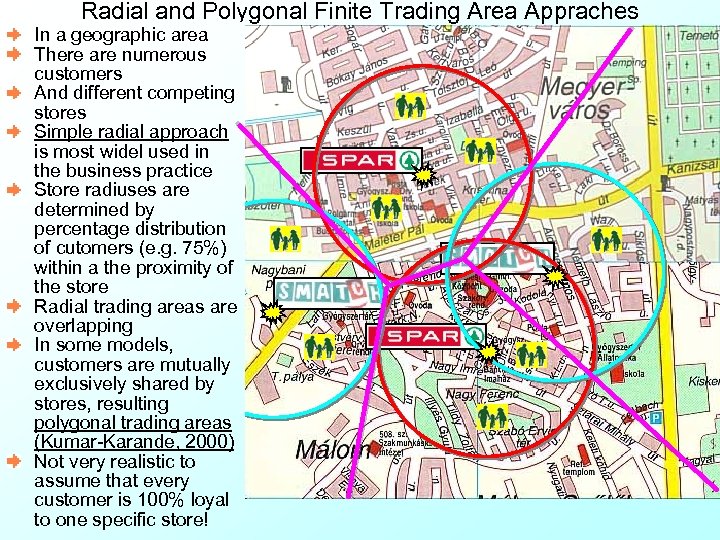
Radial and Polygonal Finite Trading Area Appraches In a geographic area There are numerous customers And different competing stores Simple radial approach is most widel used in the business practice Store radiuses are determined by percentage distribution of cutomers (e. g. 75%) within a the proximity of the store Radial trading areas are overlapping In some models, customers are mutually exclusively shared by stores, resulting polygonal trading areas (Kumar-Karande, 2000) Not very realistic to assume that every customer is 100% loyal to one specific store!
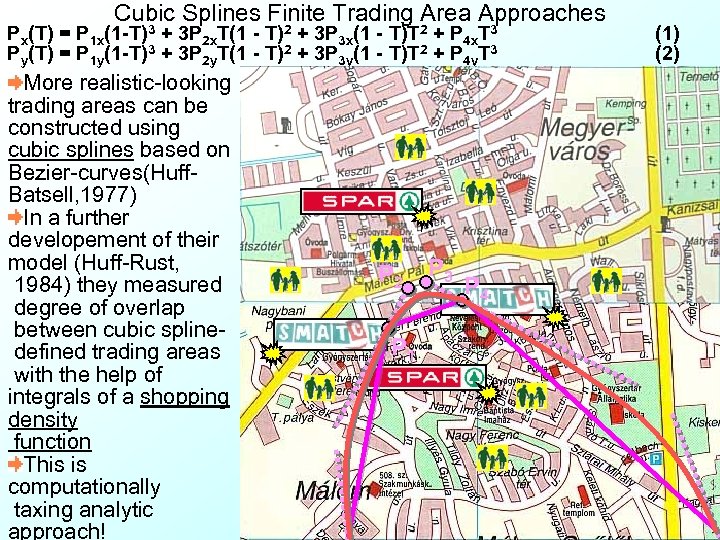
Cubic Splines Finite Trading Area Approaches Px(T) = P 1 x(1 -T)3 + 3 P 2 x. T(1 - T)2 + 3 P 3 x(1 - T)T 2 + P 4 x. T 3 Py(T) = P 1 y(1 -T)3 + 3 P 2 y. T(1 - T)2 + 3 P 3 y(1 - T)T 2 + P 4 y. T 3 More realistic-looking trading areas can be constructed using cubic splines based on Bezier-curves(Huff. Batsell, 1977) In a further developement of their model (Huff-Rust, 1984) they measured degree of overlap between cubic spline defined trading areas with the help of integrals of a shopping density function This is computationally taxing analytic approach! P 2 P 1 P 3 P 4 (1) (2)
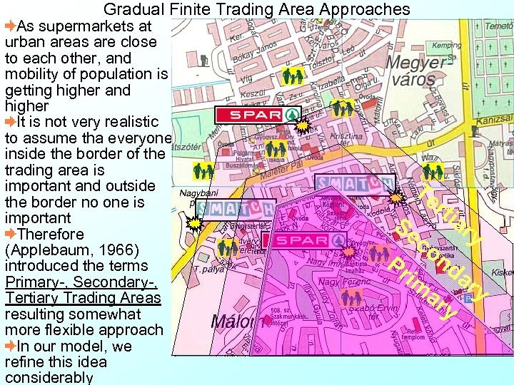
Gradual Finite Trading Area Approaches As supermarkets at urban areas are close to each other, and mobility of population is getting higher and higher It is not very realistic to assume tha everyone inside the border of the trading area is important and outside the border no one is important Therefore (Applebaum, 1966) introduced the terms Primary-, Secondary-, Tertiary Trading Areas resulting somewhat more flexible approach In our model, we refine this idea considerably Te r Se co tia ry nd im ar ar y y Pr
Content of the Presentation Significance of benchmarking stores Literature overview Infinite trading are approach: the original Huff-model Finite trading area approaches Radial Polygonal Cubic splines Gradual approaches Our store benchmarking model: Basic assumptions Objectives Input data Geocoding of stores, distance computations Analyzing satelite photos Basic equations of the model Estimation of parameters Testing of parameter estimation Benchmarking measures Practical application Evaluating estimated parameters Spatial mapping of the results Summary, References
Pauler-Trivedi-Gauri: Quasi Infinite Market Force (QIMF) Model To overcome the difficulties of mainstream finite trading area approaces, we turned back to the original Huff-model: We use Huff-like infinite market force functions for fine representation of graduality, But shortcomings of the original model are corrected with the help of extensive use of loyalty card data, census data and syndicated supermarket researches. Our model uses more extensive data than mainstream finite trading area models, but its computational requirement is considerably lower. In our experience, the extra data we require is usually readily available for the management of supermarket chains, just they sometimes do not know how to use it effectively The computational efficiency helps them to run the model in a practical application, for hundreeds of stores, thousands of competitors, and millions of customers, while usual mainstream models are applied on hundreeds of customers and 1 -2 stores.
Pauler-Trivedi-Gauri: Quasi Infinite Market Force (QIMF) Model Basic assumptions: The model can be used for decision support of managers of our supermarket chain, Our chain strongly competes with other chains on a given target market. The network of roads at the target market is dense. Distances or average traveling times can be measured by using internet-based route planner software Distances of stores and customers in the model do not have to comply triangle-inequalties The target market has different districts with different population density and income. Performances of the individal supermarkets are influenced by both quality of their management and their competitive environment.

Pauler-Trivedi-Gauri: Quasi Infinite Market Force (QIMF) Model We want to evaulate: Performaces of the individual stores: are they selling well or inferior? Additionally, we have to consider: how hard is their competition? Moreover, what is the buying power of the districts of the target market nearby them? How well can our chain cover those districts in the competiton? On which stores and districts we should concentrate our limited marketing and development resources? Which store features we should improve? How important they are for the customers? Which chains are the most dangerous competitors? Where to build or where to buy a new unit of the chain?
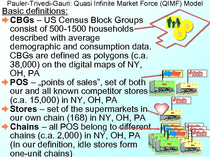
Pauler-Trivedi-Gauri: Quasi Infinite Market Force (QIMF) Model Basic definitions: CBGs – US Census Block Groups consist of 500 -1500 households described with average demographic and consumption data. CBGs are defined as polygons (c. a. 38, 000) on the digital maps of NY, OH, PA POS – „points of sales”, set of both our and all known competitor stores (c. a. 15, 000) in NY, OH, PA Stores – set of the supermarkets in our own chain (168) in NY, OH, PA Chains – all POS belong to different chains (c. a. 2, 000) in NY, OH, PA (In our definition, idle stores form one-unit chains) $ $ Big. Buy Po. Ps Big. Buy Po. Ps
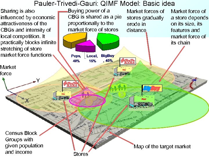
Pauler-Trivedi-Gauri: QIMF Model: Basic idea Sharing is also influenced by economic attractiveness of the CBGs and intensity of local competition. It practically blocks infinite stretching of store market force functions Buying power of a CBG is shared as a pie proportionally to the market force of stores X Census Block Groups with given population and income Market force of a store depends on its size, its features and market force of its chain Po. Ps Market force Y Market forces of stores gradually erode in distance Po. Ps $ $ $ Big. Buy Map of the target market Stores
Pauler-Trivedi-Gauri: QIMF Model: Demographic inputs CBG data from Bureau of Labor Statistics: $ Potential sales(CBG), $/week – By-category $ consumption of the population of the CBG Population density(CBG), n/sqmile – population of the CBG divided with its geographical area Education(CBG), years – average years of education of the population of CBG Age(CBG), years – average of the population of the CBG Family. Size(CBG), n – average family size of the households of the CBG Income(CBG), $/year – average yearly gross income of the households of the CBG Distance(POS, CBG), miles – There are 2 alternatives: Exact: Average travel time between POS and CBG is determined with the help of internet-based route planner software. The model does not require distances to comply triangle-inequalties Simple: Addresses of POS are geocoded, Euclidean distance is computed between their (x, y) coordinate and the centroid of the polygon of the CBG. As road network in target are was dense and high quality, we chose this option:
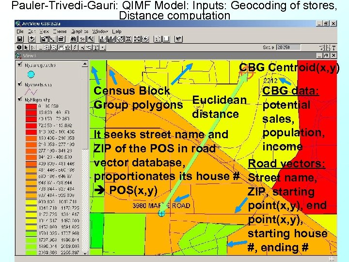
Pauler-Trivedi-Gauri: QIMF Model: Inputs: Geocoding of stores, Distance computation CBG Centroid(x, y) Census Block Group polygons Euclidean distance CBG data: potential sales, population, It seeks street name and income ZIP of the POS in road vector database, Road vectors: proportionates its house # Street name, POS(x, y) ZIP, starting point(x, y), end point(x, y), starting house #, ending #
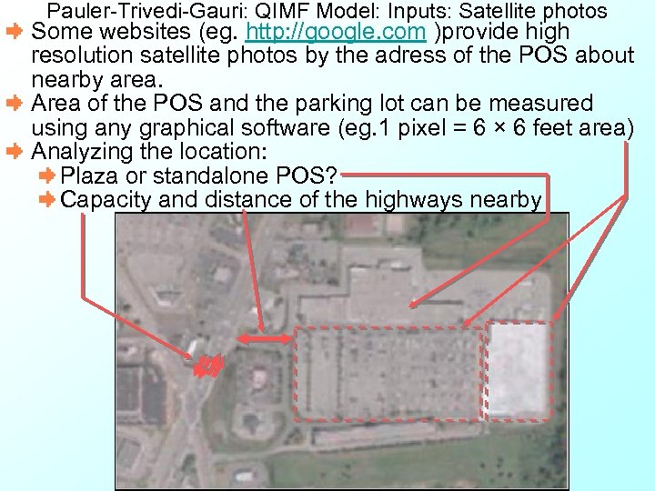
Pauler-Trivedi-Gauri: QIMF Model: Inputs: Satellite photos Some websites (eg. http: //google. com )provide high resolution satellite photos by the adress of the POS about nearby area. Area of the POS and the parking lot can be measured using any graphical software (eg. 1 pixel = 6 × 6 feet area) Analyzing the location: Plaza or standalone POS? Capacity and distance of the highways nearby
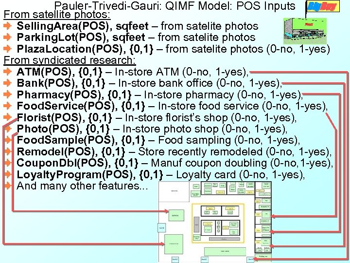
Pauler-Trivedi-Gauri: QIMF Model: POS Inputs Big. Buy From satellite photos: Selling. Area(POS), sqfeet – from satelite photos Parking. Lot(POS), sqfeet – from satelite photos Plaza. Location(POS), {0, 1} – from satelite photos (0 -no, 1 -yes) From syndicated research: ATM(POS), {0, 1} – In-store ATM (0 -no, 1 -yes), Bank(POS), {0, 1} – In-store bank office (0 -no, 1 -yes), Pharmacy(POS), {0, 1} – In-store pharmacy (0 -no, 1 -yes), Food. Service(POS), {0, 1} – In-store food service (0 -no, 1 -yes), Florist(POS), {0, 1} – In-store florist’s shop (0 -no, 1 -yes), Photo(POS), {0, 1} – In-store photo shop (0 -no, 1 -yes), Food. Sample(POS), {0, 1} – Food sampling (0 -no, 1 -yes), Remodel(POS), {0, 1} – Store recently remodeled (0 -no, 1 -yes), Coupon. Dbl(POS), {0, 1} – Manuf coupon doubling (0 -no, 1 -yes), Loyalty. Program(POS), {0, 1} – Loyalty card (0 -no, 1 -yes), And many other features. . .
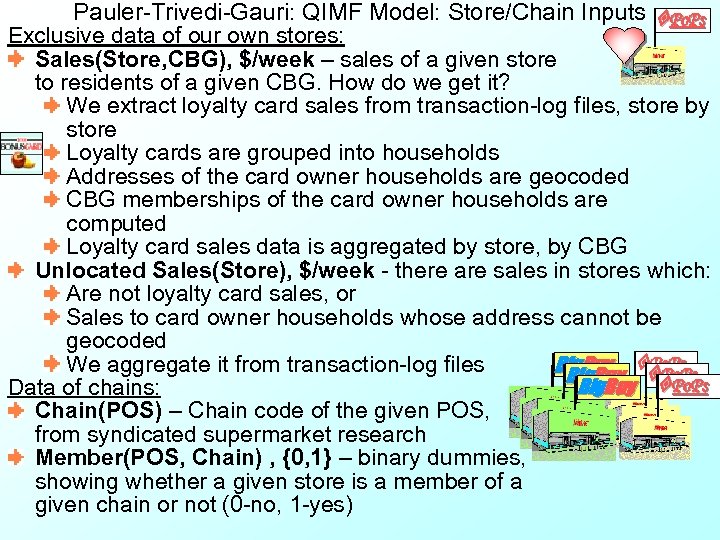
Pauler-Trivedi-Gauri: QIMF Model: Store/Chain Inputs Po. Ps Exclusive data of our own stores: Sales(Store, CBG), $/week – sales of a given store to residents of a given CBG. How do we get it? We extract loyalty card sales from transaction-log files, store by store Loyalty cards are grouped into households Addresses of the card owner households are geocoded CBG memberships of the card owner households are computed Loyalty card sales data is aggregated by store, by CBG Unlocated Sales(Store), $/week - there are sales in stores which: Are not loyalty card sales, or Sales to card owner households whose address cannot be geocoded Po. Ps We aggregate it from transaction-log files Big. Buy Po. Ps Big. Buy Po. Ps Data of chains: Chain(POS) – Chain code of the given POS, from syndicated supermarket research Member(POS, Chain) , {0, 1} – binary dummies, showing whether a given store is a member of a given chain or not (0 -no, 1 -yes)
Content of the Presentation Significance of benchmarking stores Literature overview Infinite trading are approach: the original Huff-model Finite trading area approaches Radial Polygonal Cubic splines Gradual approaches Our store benchmarking model: Basic assumptions Objectives Input data Geocoding of stores, distance computations Analyzing satelite photos Basic equations of the model Estimation of parameters Testing of parameter estimation Benchmarking measures Practical application Evaluating estimated parameters Spatial mapping of the results Summary, References
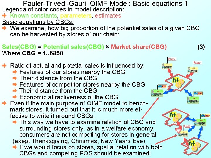
Pauler-Trivedi-Gauri: QIMF Model: Basic equations 1 Legenda of color codes in model description: Known constants, parameters, estimates Basic equations by CBGs: We examine, how big proportion of the potential sales of a given CBG can be harvested by stores of our chain: Sales(CBG) = Potential sales(CBG) × Market share(CBG) (3) Where CBG = 1. . 6850 Ratio of actual and potetial sales is influenced by: Features of our stores nearby the CBG Their distance from the CBG Features of competitor stores nearby the CBG Their distance from the CBG Economic attractiveness of the CBG Even if the main purpose of QIMF model to benchmark stores, it turned out that it is much more effective to write it around CBGs: This way we have to examine relation of CBG and surrounding stores only, as in a welfare economy, consumers are not competing for stores in general (exept Thanksgiving, Chrismas, New Years Eve) If we would focus on stores, spatial relation with both CBGs and competing POS should be examined! $ $ $
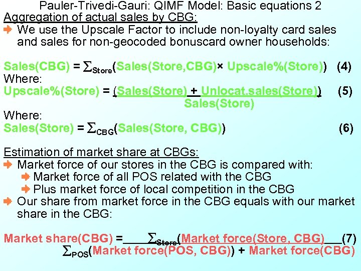
Pauler-Trivedi-Gauri: QIMF Model: Basic equations 2 Aggregation of actual sales by CBG: We use the Upscale Factor to include non-loyalty card sales and sales for non-geocoded bonuscard owner households: Sales(CBG) = Store(Sales(Store, CBG)× Upscale%(Store)) (4) Where: Upscale%(Store) = (Sales(Store) + Unlocat. sales(Store)) (5) Sales(Store) Where: Sales(Store) = CBG(Sales(Store, CBG)) (6) Estimation of market share at CBGs: Market force of our stores in the CBG is compared with: Market force of all POS related with the CBG Plus market force of local competition in the CBG Our share from market force in the CBG equals with our market share in the CBG: Market share(CBG) = Store(Market force(Store, CBG) (7) POS(Market force(POS, CBG)) + Market force(CBG)
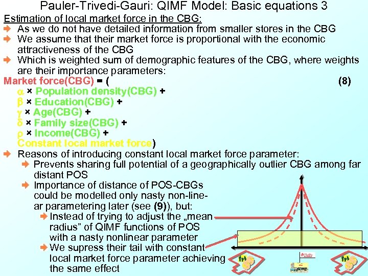
Pauler-Trivedi-Gauri: QIMF Model: Basic equations 3 Estimation of local market force in the CBG: As we do not have detailed information from smaller stores in the CBG We assume that their market force is proportional with the economic attractiveness of the CBG Which is weighted sum of demographic features of the CBG, where weights are their importance parameters: Market force(CBG) = ( (8) a × Population density(CBG) + b × Education(CBG) + g × Age(CBG) + d × Family size(CBG) + r × Income(CBG) + Constant local market force) Reasons of introducing constant local market force parameter: Prevents sharing full potential of a geographically outlier CBG among far distant POS Importance of distance of POS-CBGs could be modelled only nasty non-linear parametering later (see (9)), but: Instead of trying to adjust the „mean radius” of QIMF functions of POS with a nasty nonlinear parameter We supress their tail with constant local market force parameter achieving $ $ the same effect
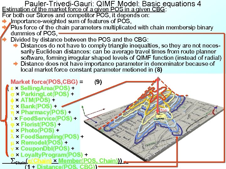
Pauler-Trivedi-Gauri: QIMF Model: Basic equations 4 Estimation of the market force of a given POS in a given CBG: For both our Stores and competitor POS, it depends on: Importance-weighted sum of features of POS, Plus force of the chain parameters multiplicated with chain membersip binary dummies of POS, Divided by distance between the POS and the CBG: Distances do not have to comply triangle inequalties, so they are not necessarily Euclidean distances: can be average travel times from route planner software, forming irregular shaped levels of QIMF function (instead of radial) Distance does not have importance parameter in denominator because of local market force constant parameter metioned in (8) Market force(POS, CBG) = (9) ( e × Selling. Area(POS) + s × Parking. Lot(POS) + f × ATM(POS) + c × Bank(POS) + h × Pharmacy(POS) + i × Food. Service(POS) + j × Florist(POS) + k × Photo(POS) + l × Food. Sampling(POS) + m × Remodel(POS) + n × Coupon. Dbl(POS) + o × Loyalty. Program(POS) + Chain(p(Chain) × Member(POS, Chain))). (1 + Distance(POS, CBG))
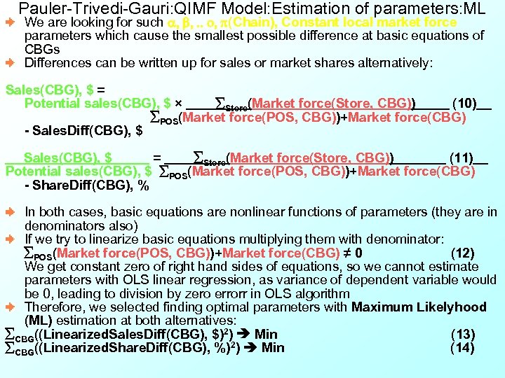
Pauler-Trivedi-Gauri: QIMF Model: Estimation of parameters: ML We are looking for such a, b, . . o, p(Chain), Constant local market force parameters which cause the smallest possible difference at basic equations of CBGs Differences can be written up for sales or market shares alternatively: Sales(CBG), $ = Potential sales(CBG), $ × Store(Market force(Store, CBG)) (10) POS(Market force(POS, CBG))+Market force(CBG) - Sales. Diff(CBG), $ Sales(CBG), $ = Store(Market force(Store, CBG)) (11) Potential sales(CBG), $ POS(Market force(POS, CBG))+Market force(CBG) - Share. Diff(CBG), % In both cases, basic equations are nonlinear functions of parameters (they are in denominators also) If we try to linearize basic equations multiplying them with denominator: POS(Market force(POS, CBG))+Market force(CBG) ≠ 0 (12) We get constant zero of right hand sides of equations, so we cannot estimate parameters with OLS linear regression, as variance of dependent variable would be 0, leading to division by zero errorr in OLS algorithm Therefore, we selected finding optimal parameters with Maximum Likelyhood (ML) estimation at both alternatives: CBG((Linearized. Sales. Diff(CBG), $)2) Min (13) CBG((Linearized. Share. Diff(CBG), %)2) Min (14)
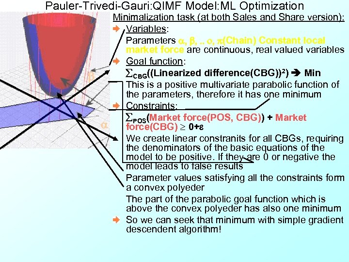
Pauler-Trivedi-Gauri: QIMF Model: ML Optimization b a Minimalization task (at both Sales and Share version): Variables: Parameters a, b, . . o, p(Chain) Constant local market force are continuous, real valued variables Goal function: CBG((Linearized difference(CBG))2) Min This is a positive multivariate parabolic function of the parameters, therefore it has one minimum Constraints: POS(Market force(POS, CBG)) + Market force(CBG) 0+e We create linear constranits for all CBGs, requiring the denominators of the basic equations of the model to be positive. If they are 0 or negative the model leads to false results Parameter values satisfying all the constraints form a convex polyeder The part of the parabolic goal function which is above the convex polyeder has also one minimum So we can seek that minimum with simple gradient descendent algorithm!
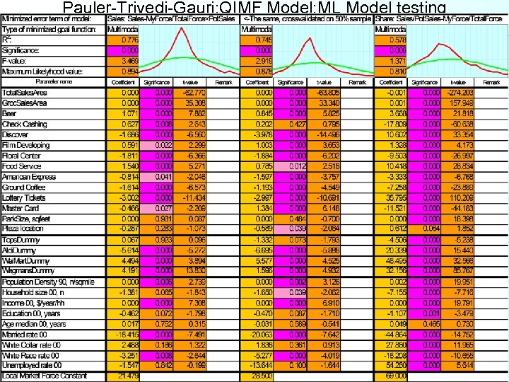
Pauler-Trivedi-Gauri: QIMF Model: ML Model testing
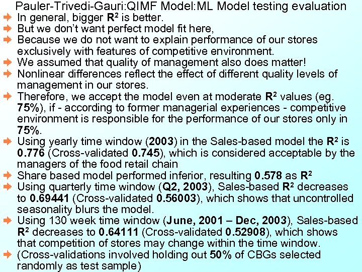
Pauler-Trivedi-Gauri: QIMF Model: ML Model testing evaluation In general, bigger R 2 is better. But we don’t want perfect model fit here, Because we do not want to explain performance of our stores exclusively with features of competitive environment. We assumed that quality of management also does matter! Nonlinear differences reflect the effect of different quality levels of management in our stores. Therefore, we accept the model even at moderate R 2 values (eg. 75%), if - according to former managerial experiences - competitive environment is responsible for the performance of our stores only in 75%. Using yearly time window (2003) in the Sales-based model the R 2 is 0. 776 (Cross-validated 0. 745), which is considered acceptable by the managers of the food retail chain Share based model performed inferior, resulting 0. 578 as R 2 Using quarterly time window (Q 2, 2003), Sales-based R 2 decreases to 0. 69441 (Cross-validated 0. 56003), which shows that uncontrolled seasonality blurs the model. Using 130 week time window (June, 2001 – Dec, 2003), Sales-based R 2 decreases to 0. 64111 (Cross-validated 0. 52908), which shows that competition of stores may change within the time window. (Cross-validations involved holding out 50% of CBGs selected randomly as test sample)
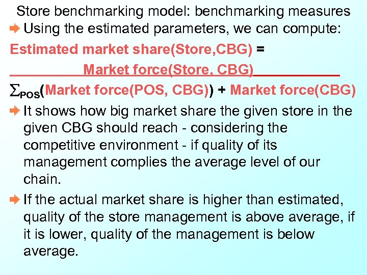
Store benchmarking model: benchmarking measures Using the estimated parameters, we can compute: Estimated market share(Store, CBG) = Market force(Store, CBG) POS(Market force(POS, CBG)) + Market force(CBG) It shows how big market share the given store in the given CBG should reach - considering the competitive environment - if quality of its management complies the average level of our chain. If the actual market share is higher than estimated, quality of the store management is above average, if it is lower, quality of the management is below average.
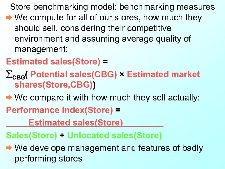
Store benchmarking model: benchmarking measures We compute for all of our stores, how much they should sell, considering their competitive environment and assuming average quality of management: Estimated sales(Store) = CBG( Potential sales(CBG) × Estimated market shares(Store, CBG)) We compare it with how much they sell actually: Performance index(Store) = Estimated sales(Store) Sales(Store) + Unlocated sales(Store) We develope management and features of badly performing stores
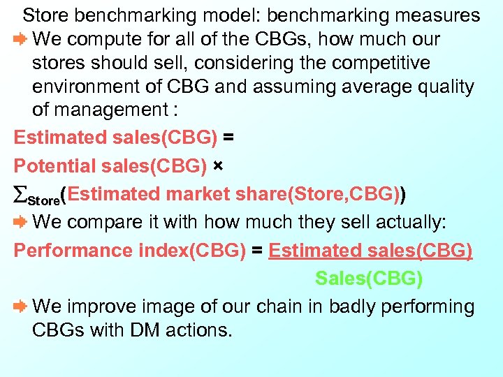
Store benchmarking model: benchmarking measures We compute for all of the CBGs, how much our stores should sell, considering the competitive environment of CBG and assuming average quality of management : Estimated sales(CBG) = Potential sales(CBG) × Store(Estimated market share(Store, CBG)) We compare it with how much they sell actually: Performance index(CBG) = Estimated sales(CBG) Sales(CBG) We improve image of our chain in badly performing CBGs with DM actions.
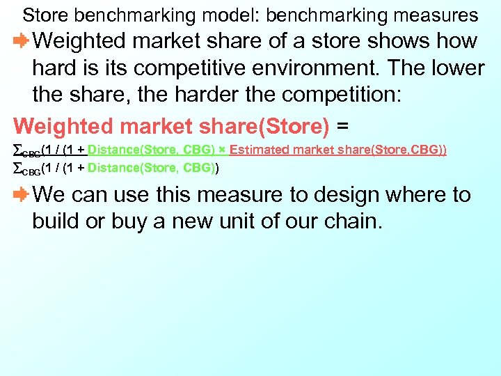
Store benchmarking model: benchmarking measures Weighted market share of a store shows how hard is its competitive environment. The lower the share, the harder the competition: Weighted market share(Store) = CBG(1 / (1 + Distance(Store, CBG) × Estimated market share(Store, CBG)) CBG(1 / (1 + Distance(Store, CBG)) We can use this measure to design where to build or buy a new unit of our chain.
Content of the Presentation Significance of benchmarking stores Literature overview Infinite trading are approach: the original Huff-model Finite trading area approaches Radial Polygonal Cubic splines Gradual approaches Our store benchmarking model: Basic assumptions Objectives Input data Geocoding of stores, distance computations Analyzing satelite photos Basic equations of the model Estimation of parameters Testing of parameter estimation Benchmarking measures Practical application Evaluating estimated parameters Spatial mapping of the results Summary, References
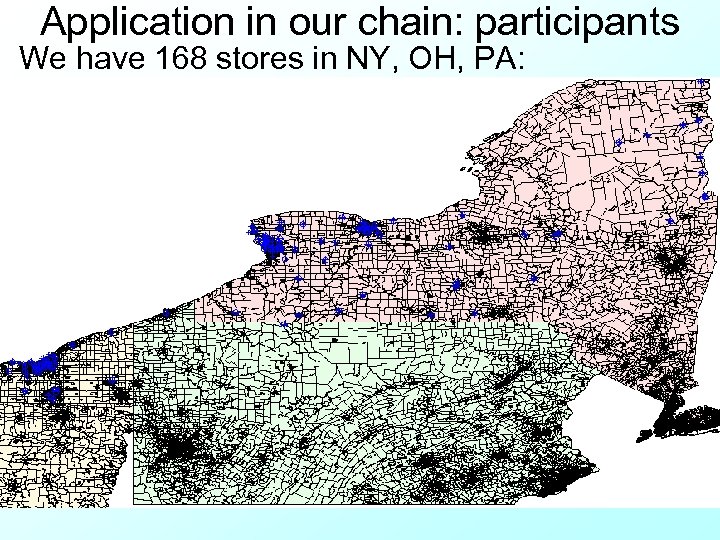
Application in our chain: participants We have 168 stores in NY, OH, PA:
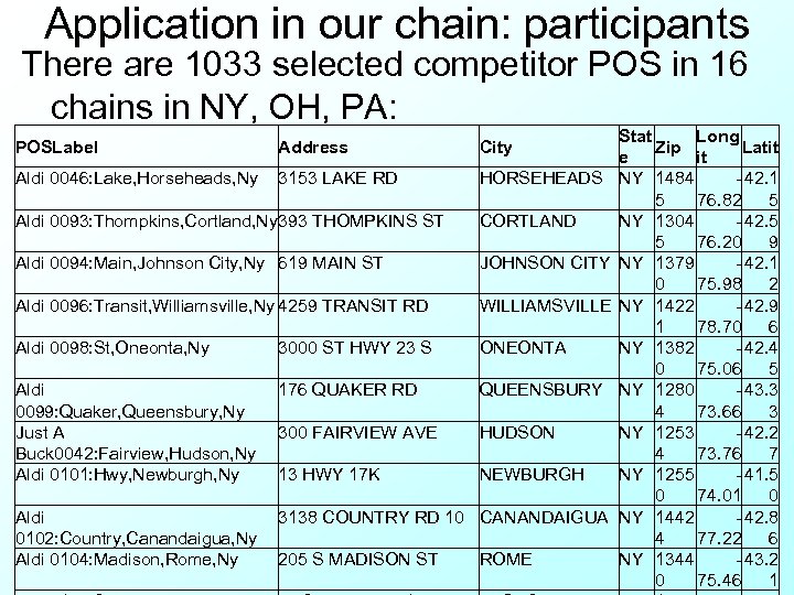
Application in our chain: participants There are 1033 selected competitor POS in 16 chains in NY, OH, PA: POSLabel Address City Aldi 0046: Lake, Horseheads, Ny 3153 LAKE RD HORSEHEADS Aldi 0093: Thompkins, Cortland, Ny 393 THOMPKINS ST CORTLAND Aldi 0094: Main, Johnson City, Ny 619 MAIN ST JOHNSON CITY Aldi 0096: Transit, Williamsville, Ny 4259 TRANSIT RD WILLIAMSVILLE Aldi 0098: St, Oneonta, Ny 3000 ST HWY 23 S ONEONTA Aldi 0099: Quaker, Queensbury, Ny Just A Buck 0042: Fairview, Hudson, Ny Aldi 0101: Hwy, Newburgh, Ny 176 QUAKER RD QUEENSBURY 300 FAIRVIEW AVE HUDSON 13 HWY 17 K NEWBURGH Aldi 0102: Country, Canandaigua, Ny Aldi 0104: Madison, Rome, Ny 3138 COUNTRY RD 10 CANANDAIGUA 205 S MADISON ST ROME Stat Long Zip Latit e it NY 1484 - 42. 1 5 76. 82 5 NY 1304 - 42. 5 5 76. 20 9 NY 1379 - 42. 1 0 75. 98 2 NY 1422 - 42. 9 1 78. 70 6 NY 1382 - 42. 4 0 75. 06 5 NY 1280 - 43. 3 4 73. 66 3 NY 1253 - 42. 2 4 73. 76 7 NY 1255 - 41. 5 0 74. 01 0 NY 1442 - 42. 8 4 77. 22 6 NY 1344 - 43. 2 0 75. 46 1
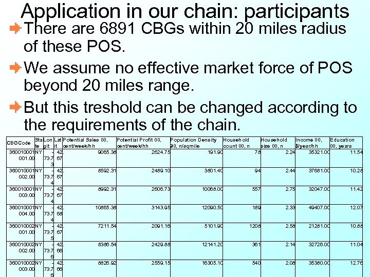
Application in our chain: participants There are 6891 CBGs within 20 miles radius of these POS. We assume no effective market force of POS beyond 20 miles range. But this treshold can be changed according to the requirements of the chain. Sta Lon Lat Potential Sales 00, Potential Profit 00, Population Density Household Income 00, Education te git it cent/week/hh 90, n/sqmile count 00, n size 00, n $/year/hh 00, years 360010001 NY - 42. 9065. 38 2624. 75 191. 90 78 2. 24 35321. 00 11. 54 001. 00 73. 7 67 3 360010001 NY - 42. 8592. 31 2489. 10 3801. 40 94 2. 44 37681. 00 10. 28 002. 00 73. 7 67 4 360010001 NY - 42. 8992. 31 2606. 73 10068. 00 557 2. 75 32047. 00 11. 42 003. 00 73. 7 67 4 360010001 NY - 42. 10865. 38 3143. 95 12090. 50 189 2. 33 49407. 00 12. 07 004. 00 73. 7 68 4 360010002 NY - 42. 7211. 54 2091. 16 5101. 90 1208 2. 58 21281. 00 10. 88 001. 00 73. 7 67 5 360010002 NY - 42. 8386. 54 2429. 88 12141. 20 361 2. 14 32726. 00 11. 04 002. 00 73. 7 66 6 360010002 NY - 42. 8826. 92 2559. 15 16305. 10 540 2. 08 35380. 00 12. 76 003. 00 73. 7 66 CBGCode
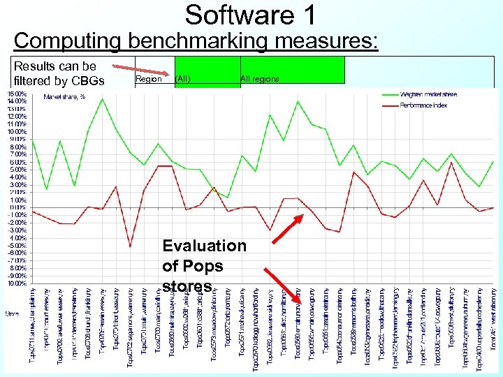
Software 1 Computing benchmarking measures: Results can be filtered by CBGs and regions Region (All) All regions Store Label Tops 0221: erie, derby, ny Tops 0261: bway, alden, ny Tops 0838: center, brunswick, oh Tops 0021: stransit, lockport, ny Tops 0508: wst, sfulton, ny Tops 0119: grandisld, grandisland, ny Tops 0700: main, corinth, ny Tops 0650: nelmira, sayre, pa Tops 0712: route 9, cheertown, ny Tops 0034: vineyard, dunkirk, ny Tops 0236: spark, hamburg, ny Tops 0539: wmorris, bath, ny Tops 0118: grey, eaurora, ny Tops 0233: cascade, springville, ny Tops 0814: walker, avonlake, oh Tops 0517: route 281, cortland, ny CBGCode (All) Data Store 221 261 838 21 508 Potential Sales, Actual Sales, $/week 2, 098, 818. 42 2, 679, 594. 35 4, 359, 799. 78 4, 735, 092. 91 2, 277, 325. 31 5, 621, 555. 24 1, 549, 620. 61 2, 774, 692. 49 1, 691, 217. 74 2, 106, 666. 39 3, 117, 567. 91 Estimated Sales, $/week Residual Sales, $/week Estimate Market d Market Share, Residual, % % % 7. 52% 3. 79% 3. 73% 6. 04% 2. 86% 3. 18% 6. 50% 3. 28% 3. 22% 8. 90% 4. 45% 5. 62% 4. 09% 1. 53% 157, 804. 73 161, 715. 62 283, 269. 93 421, 602. 02 127, 955. 63 79, 445. 48 78, 359. 25 76, 542. 18 85, 173. 44 142, 941. 79 140, 328. 14 210, 762. 12 210, 839. 90 93, 156. 49 34, 799. 14 405, 480. 27 112, 128. 54 143, 713. 62 72, 138. 70 89, 057. 08 205, 923. 53 44, 164. 18 139, 622. 40 10. 61% 20, 808. 23 14, 840. 70 9. 03% 32, 109. 44 26, 831. 48 10. 54% 3, 503. 70 4, 711. 18 8. 21% 124, 119. 92 74, 330. 43 9. 29% 254, 068. 15 151, 412. 12 7. 21% 81, 777. 06 30, 351. 48 7. 24% 62, 128. 79 81, 584. 83 5. 18% 22, 226. 16 49, 912. 54 4. 27% 101, 259. 32 -12, 202. 24 4. 23% 131, 885. 24 74, 038. 29 6. 61% Evaluation 183, 786. 58 1, 732, 371. 74 394, 926. 24 35, 648. 93 of Pops 559, 465. 69 58, 940. 93 100, 077. 37 8, 214. 88 stores 2, 135, 647. 26 198, 450. 36 119 700 650 712 34 236 539 118 233 814 517 2. 55% 8. 06% 5. 27% 3. 76% 5. 74% 4. 80% 3. 50% 4. 71% 5. 81% 3. 48% 4. 52% 2. 69% 5. 28% 1. 96% 2. 24% 2. 94% 1. 31% 2. 95% 4. 81% -0. 58% 4. 23% 2. 37%
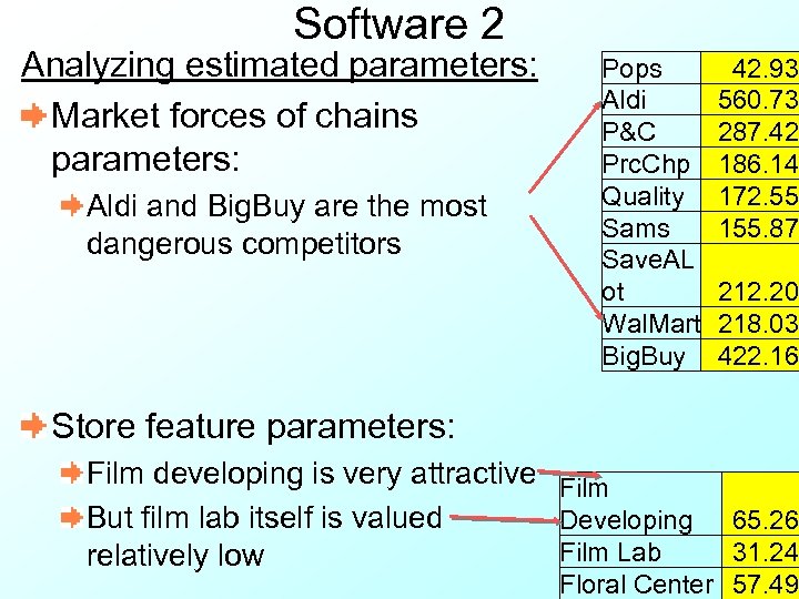
Software 2 Analyzing estimated parameters: Market forces of chains parameters: Aldi and Big. Buy are the most dangerous competitors Pops Aldi P&C Prc. Chp Quality Sams Save. AL ot Wal. Mart Big. Buy 42. 93 560. 73 287. 42 186. 14 172. 55 155. 87 212. 20 218. 03 422. 16 Store feature parameters: Film developing is very attractive Film But film lab itself is valued Developing Film Lab relatively low 65. 26 31. 24 Floral Center 57. 49
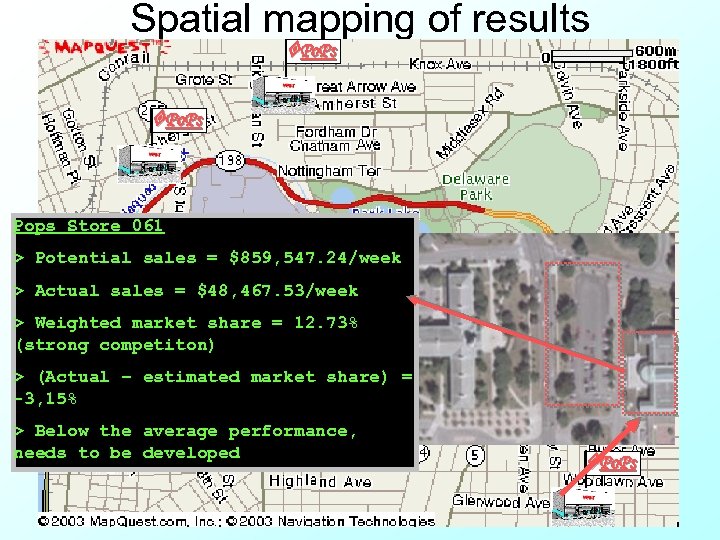
Spatial mapping of results Po. Ps Pops Store 061 > Potential sales = $859, 547. 24/week > Actual sales = $48, 467. 53/week > Weighted market share = 12. 73% (strong competiton) > (Actual – estimated market share) = -3, 15% > Below the average performance, needs to be developed Po. Ps
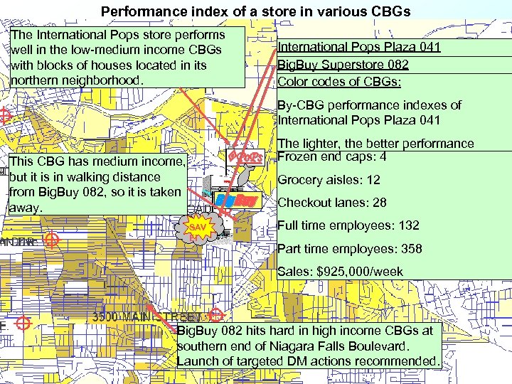
Performance index of a store in various CBGs The International Pops store performs well in the low-medium income CBGs with blocks of houses located in its northern neighborhood. This CBG has medium income, but it is in walking distance from Big. Buy 082, so it is taken away. SAV E! Po. Ps Big. Buy International Pops Plaza 041 Big. Buy Superstore 082 Latitude: +42. 991, Longitude: -78. 815 Color codes of CBGs: Latitude: +42. 989, Longitude: -78. 817 Sales area: 83, 000 sqfeet By-CBG performance indexes of Sales area: 116, 000 sqfeet Parking lot: 126, 262 sqfeet International Pops Plaza 041 Parking lot: 475, 411 sqfeet Frozen end caps: 12 The lighter, the better performance Frozen end caps: 4 Grocery aisles: 19 Grocery aisles: 12 Checkout lanes: 21 Checkout lanes: 28 Full time employees: 113 Full time employees: 132 Part time employees: 210 Part time employees: 358 Sales: $800, 000/week Sales: $925, 000/week Big. Buy 082 hits hard in high income CBGs at southern end of Niagara Falls Boulevard. Launch of targeted DM actions recommended.
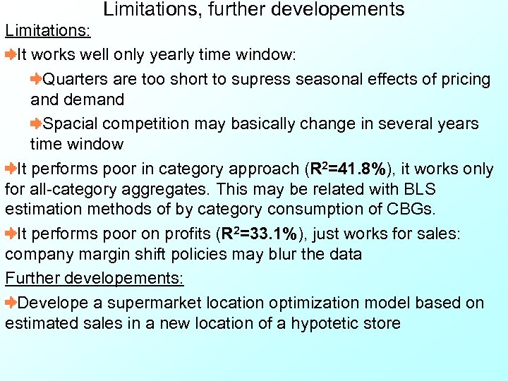
Limitations, further developements Limitations: It works well only yearly time window: Quarters are too short to supress seasonal effects of pricing and demand Spacial competition may basically change in several years time window It performs poor in category approach (R 2=41. 8%), it works only for all-category aggregates. This may be related with BLS estimation methods of by category consumption of CBGs. It performs poor on profits (R 2=33. 1%), just works for sales: company margin shift policies may blur the data Further developements: Develope a supermarket location optimization model based on estimated sales in a new location of a hypotetic store
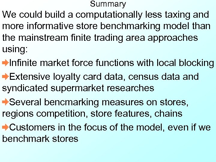
Summary We could build a computationally less taxing and more informative store benchmarking model than the mainstream finite trading area approaches using: Infinite market force functions with local blocking Extensive loyalty card data, census data and syndicated supermarket researches Several bencmarking measures on stores, regions competition, store features, chains Customers in the focus of the model, even if we benchmark stores
References 1 Achabal, Dale D. , Wilpen Gorr and Vijay Mahajan (1982), “MULTILOC: A Multiple Store Location Decision Model”, Journal of Retailing 58 (Summer), 5– 25. Applebaum, William (1966), “Methods for Determining Store Trade Areas, Market Penetration, and Potential Sales”, Journal of Marketing Research 3 (May), 127 -141. Bucklin Randolph E. and Sunil Gupta (1999), "Commercial Use of UPC Scanner Data: Industry and Academic Perspectives, " Marketing Science, 18(3) (Summer), 247 -273 Campo, K. , Gijsbrechts, E. , Goossens, T. , and Verhetsel, A. (2000), “The impact of location factors on the attractiveness and optimal space shares of product categories”, International Journal of Research in Marketing 17 (November), 255 -279. Craig, Samuel C. , Avijit Ghosh, Avijit. , and Sara Mc. Lafferty (1984), “Models of Retail Location Process: A Review”, Journal of Retailing 60 (Spring), 5– 36. Darden, Wiliam R. , and Babin, Barry J. (1994), “Exploring the Concept of Affective Quality: Expanding the Concept of Retail Personality”, Journal of Business Research 29 (February), 101– 109.
References 2 Donovan, Robert J. , and Rossiter, John (1982), “Store Atmosphere: An Environment Psychology Approach”, Journal of Retailing 58 (Spring), 34– 57. Dunn, Patrick, Robert Lusch and Myron Gable (1995), Retailing, Southwestern Publishing, Cincinnati, Ohio. Durvasula, Srinivas, Subhash Sharma, and Andrews J. Craig (1992), “Storeloc: A Retail Store Location Model Based on Managerial Judgements”, Journal of Retailing 68 (Winter), 420– 444. Gardner, Meryl P. and George J. Siomkos (1986), “Towards a Methodology for Assessing Effects of In-Store Atmospherics”, Advances in Consumer Research, Vol. 13, Ann Arbor: Association for Consumer Research, 27 -31 Ghosh, Avijit (1984), “Parameter Non-Stationarity in Retail Choice Models”, Journal of Business Research 19 (4), 425– 436. ______, and Mc. Lafferty, Sara. L (1982), “Locating Stores in Uncertain Environments: A Scenario Planning Approach”, Journal of Retailing 58 (Winter), 5– 22. ____, and ____ (1987), Location Strategies for Retail and Service Firms, Lexington Books, Lexington, MA. Goldberg, David E (1989), Genetic Algorithms in Search, Optimization, and Machine Learning, Wiley & Sons, New York, 137
References 3 Hoch, Stephen. J. , Byung Do Kim, Alan Montgomery, and Peter Rossi (1995), “Determinants of Store-Level Price Elasticity”, Journal of Marketing Research 32 (February), 17– 28. Huff, David. L. (1964), “Defining and Estimating a Trade Area”, Journal of Marketing 28 (July), 34– 38. ____ and Richard R. Batsell (1977), “Delimiting the Areal Extent of a Market Area”, Journal of Marketing Research 14 (November), 581– 585. ____ and Roland Rust (1984), “Measuring the Congruence of Market Areas”, Journal of Marketing 48 (Winter), 68– 74. Ingene, Charles A. , and Robert F. Lusch (1980), “Market Selection Decisions for Departmental Stores”, Journal of Retailing 56 (Fall), 21– 40. Jain, Arun. K. , and Vijay Mahajan (1979), “Evaluating the Competitive Environment in Retailing Using Multiplicative Competitive Interactive Models”, Research in Marketing, J. Sheth, ed. , Jain Press, Greenwich, 217– 235. Kotler, Philip (1973), “Atmospherics as a Marketing Tool”, Journal of Retailing 49 (Winter): 49– 64.
References 4 Kumar, V. , and Kiran Karande (2000), “The Effect of Retail Store Environment on Retailer Performance”, Journal of Business Research 49 (2), 167 -181. Loken and Ward, 1990 Mahajan, Vijay, Subhash Sharma, and Durvasula Srinivas (1985), “An Application of Portfolio Analysis for Identifying Attractive Retail Locations”, Journal of Retailing 61 (Winter), 19– 34. Pauler, G. – Trivedi, M. – Gauri, D. : Assessing Store Performance Equitably, EJOR, 2008 Reilly, William (1931), The Law of Retail Gravitation, Knickerbockers, New York. Reinartz, Werner and V. Kumar (1999), “Store-, Market-, and Consumer Characteristics: On the Drivers of Store Performance”, Marketing Letters 10 (1), 3 -20. Walters, Rockney, and Scott Mackenzie (1988), “A Structural Equations Analysis of the Impact of Price Promotions on Store Performance”, Journal of Marketing Research 25 (February), 51– 63. _____ and Heikki Rinne (1986), “An Empirical Investigation into the Impact of Price Promotions on Retail Store Performance”, Journal of Retailing 62 (Fall), 237– 266. Wrigley, Neil (1990), Store Choice, Store Location and Market Analysis, Routledge, London.
aea5062d91041b32cf2fff2bd3fac67e.ppt