Arbitrage Pricing Theory and Multifactor Models of Risk

Single Factor Model Returns on a security come from two sources Common macro-economic factor Firm specific events Possible common macro-economic factors Gross Domestic Product Growth Interest Rates 11 -2

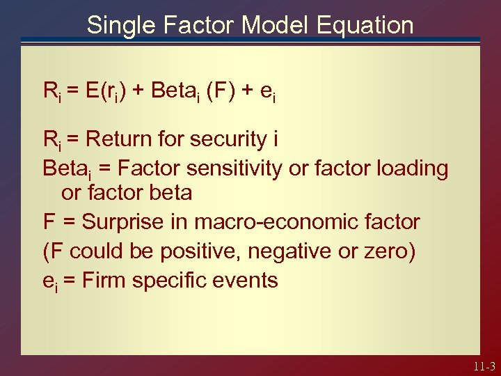
Single Factor Model Equation Ri = E(ri) + Betai (F) + ei Ri = Return for security i Betai = Factor sensitivity or factor loading or factor beta F = Surprise in macro-economic factor (F could be positive, negative or zero) ei = Firm specific events 11 -3

Multifactor Models Use more than one factor in addition to market return. Examples include gross domestic product, expected inflation, interest rates etc. Estimate a beta or factor loading for each factor using multiple regression. They can provide better descriptions of security returns. 11 -4

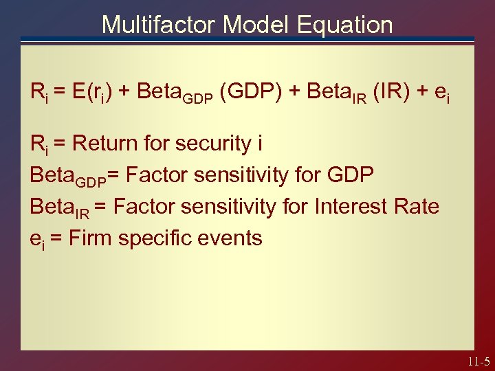
Multifactor Model Equation Ri = E(ri) + Beta. GDP (GDP) + Beta. IR (IR) + ei Ri = Return for security i Beta. GDP= Factor sensitivity for GDP Beta. IR = Factor sensitivity for Interest Rate ei = Firm specific events 11 -5

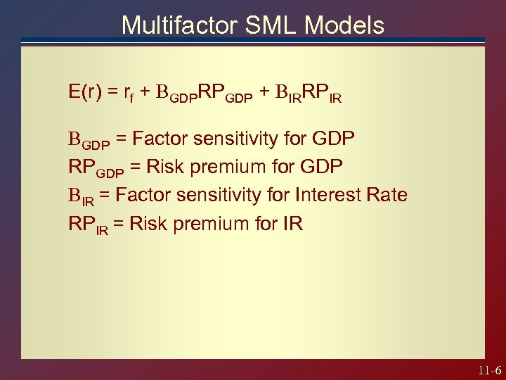
Multifactor SML Models E(r) = rf + BGDPRPGDP + BIRRPIR BGDP = Factor sensitivity for GDP RPGDP = Risk premium for GDP BIR = Factor sensitivity for Interest Rate RPIR = Risk premium for IR 11 -6

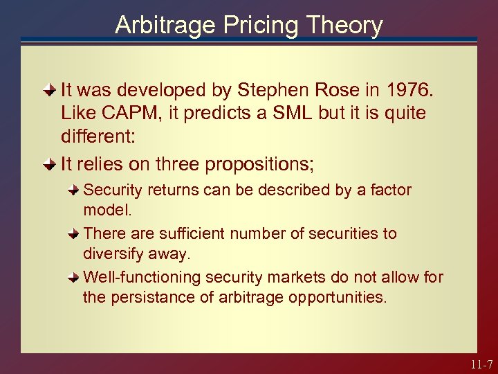
Arbitrage Pricing Theory It was developed by Stephen Rose in 1976. Like CAPM, it predicts a SML but it is quite different: It relies on three propositions; Security returns can be described by a factor model. There are sufficient number of securities to diversify away. Well-functioning security markets do not allow for the persistance of arbitrage opportunities. 11 -7

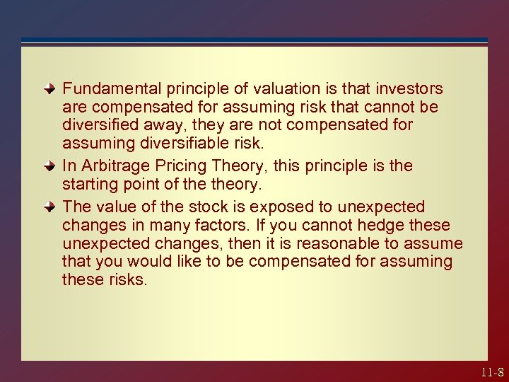
Fundamental principle of valuation is that investors are compensated for assuming risk that cannot be diversified away, they are not compensated for assuming diversifiable risk. In Arbitrage Pricing Theory, this principle is the starting point of theory. The value of the stock is exposed to unexpected changes in many factors. If you cannot hedge these unexpected changes, then it is reasonable to assume that you would like to be compensated for assuming these risks. 11 -8

An arbitrage portfolio is a portfolio that requires zero wealth and eliminated all unsystematic and systematic risk. The basic principle is that such a portfolio must also have zero return; otherwise, it offers an arbitrage opportunity. 11 -9

To create an arbitrage portfolio we must eliminate all systematic and unsystematic risk. Unsystematic risk can be eliminated simply by having many securities in the portfolio. To achive this we must have a large number of securities available. 11 -10

The next requirement of a “zero wealth portfolio; from your existing position you can construct this portfolio without contributing or withdrawing any cash. That is achievied by taking both long and short positions that offset each other in costs and revenues. This requires you to be able to short sale. In efficient markets, profitable arbitrage opportunities will quickly disappear. 11 -11

The Law of One Price states that if two assets are equivalent in all economically relevant respects, then they should have the same market price. If investors observe a violation of this Law, they will engage in arbitrage activity-simultaneolusly buying the assets where it is cheap and selling it where it is expensive. In the process, they will bid up the price where it is low and force it down where it is high until the arbitrage opportunity is eliminated. 11 -12

The important property of the risk-free arbitrage portfolio is that any investor, regardless of risk-aversion or wealt, will want to take an infinite position in it. Because large positions will quickly force prices up or down until the opportunity vanishes. 11 -13

According to CAPM, all investors hold meanvariance efficient portfolios. If a security is mispriced, the investors will buy underpriced and away from overpriced securities in their portfolios. Pressure on equilibrium prices results from many investors shifting their porfolios, each by a relatively small enough. According to the APT, a few investors who identify an arbitrage opportunity will mobilize large dollar amounts and quickly restore equilibrium. 11 -14

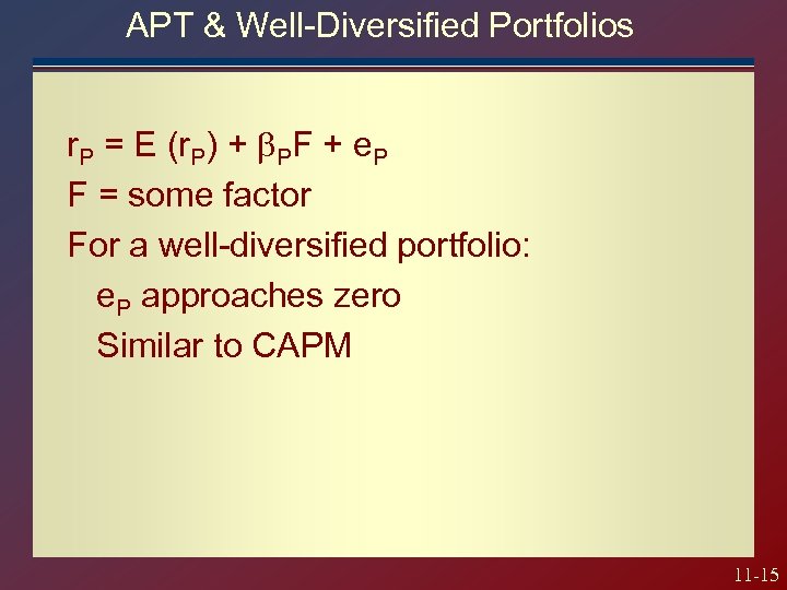
APT & Well-Diversified Portfolios r. P = E (r. P) + b. PF + e. P F = some factor For a well-diversified portfolio: e. P approaches zero Similar to CAPM 11 -15

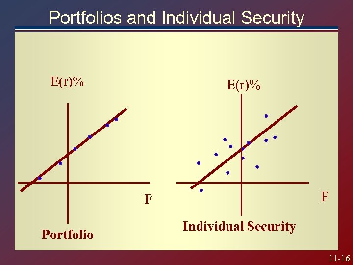
Portfolios and Individual Security E(r)% F F Portfolio Individual Security 11 -16

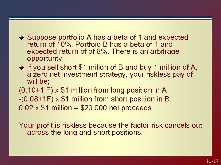
Suppose portfolio A has a beta of 1 and expected return of 10%. Portfoio B has a beta of 1 and expected return of of 8%. There is an arbitrage opportunty: If you sell short $1 milion of B and buy 1 million of A, a zero net investment strategy, your riskless pay of will be; (0. 10+1 F) x $1 million from long position in A -(0. 08+1 F) x $1 million from short position in B. 0. 02 x $1 million = $20, 000 net proceeds Your profit is riskless because the factor risk cancels out across the long and short positions. 11 -17

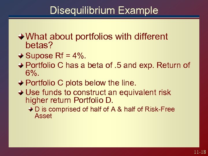
Disequilibrium Example What about portfolios with different betas? Supose Rf = 4%. Portfolio C has a beta of. 5 and exp. Return of 6%. Portfolio C plots below the line. Use funds to construct an equivalent risk higher return Portfolio D. D is comprised of half of A & half of Risk-Free Asset 11 -18

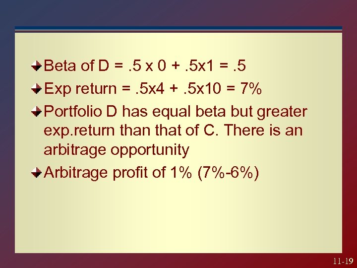
Beta of D =. 5 x 0 +. 5 x 1 =. 5 Exp return =. 5 x 4 +. 5 x 10 = 7% Portfolio D has equal beta but greater exp. return that of C. There is an arbitrage opportunity Arbitrage profit of 1% (7%-6%) 11 -19

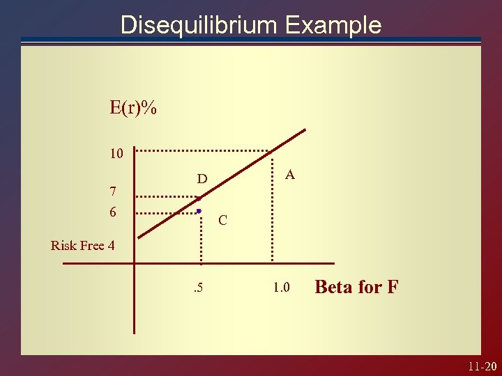
Disequilibrium Example E(r)% 10 7 6 A D C Risk Free 4. 5 1. 0 Beta for F 11 -20

» APT with Market Index Portfolio E(r)% M [E(r. M) - rf] Market Risk Premium Risk Free 1. 0 Beta (Market Index) 11 -21

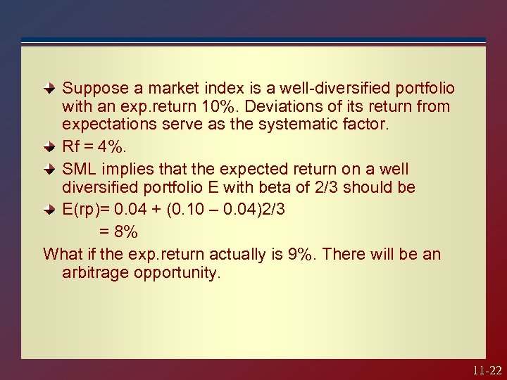
Suppose a market index is a well-diversified portfolio with an exp. return 10%. Deviations of its return from expectations serve as the systematic factor. Rf = 4%. SML implies that the expected return on a well diversified portfolio E with beta of 2/3 should be E(rp)= 0. 04 + (0. 10 – 0. 04)2/3 = 8% What if the exp. return actually is 9%. There will be an arbitrage opportunity. 11 -22

We can construct a new portfolio that has the same Beta of E. 1/3 of Rf and 2/3 of market portfolio. B=1/3 x 0+ 2/3 x 1= 2/3 E(rp) = 1/3 x 0. 04+2/3 x 0, 10=0, 08 Buy $1 of portfolio E and sell $1 portfolio invested in 1/3 in rf and 2/3 in market index. $1 x (0. 09) -$1 x (0, 08) $1 x 0. 01 Deviation of expected return from the SML(9%-8%) 11 -23

APT and CAPM Compared APT applies to well diversified portfolios and not necessarily to individual stocks. With APT it is possible for some individual stocks to be mispriced - not lie on the SML. APT is more general in that it gets to an expected return and beta relationship without the assumption of the market portfolio. APT can be extended to multifactor models. 11 -24

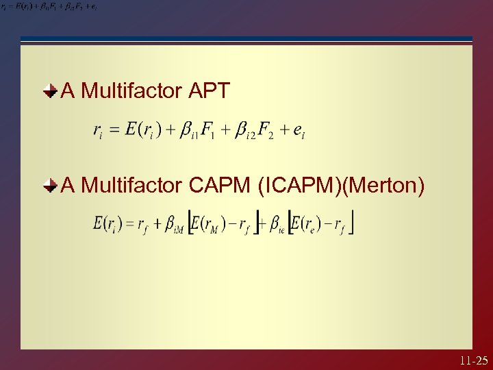
A Multifactor APT A Multifactor CAPM (ICAPM)(Merton) 11 -25