Approximation Algorithms for Non-Uniform Buy-at-Bulk Network Design Problems

Approximation Algorithms for Non-Uniform Buy-at-Bulk Network Design Problems Guy Kortsarz Rutgers University, Camden, NJ Joint work with C. Chekuri (Bell Labs) M. T. Hajiaghayi (CMU) M. R. Salavatipour (University of Alberta)

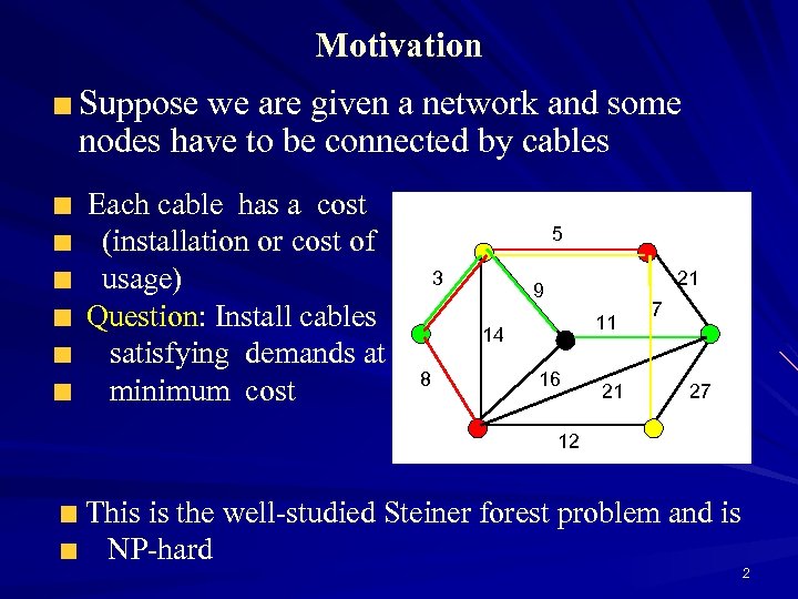
Motivation Suppose we are given a network and some nodes have to be connected by cables Each cable has a cost (installation or cost of usage) Question: Install cables satisfying demands at minimum cost 5 3 14 8 21 9 10 11 16 21 7 27 12 This is the well-studied Steiner forest problem and is NP-hard 2

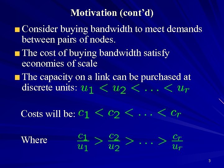
Motivation (cont’d) Consider buying bandwidth to meet demands between pairs of nodes. The cost of buying bandwidth satisfy economies of scale The capacity on a link can be purchased at discrete units: Costs will be: Where 3

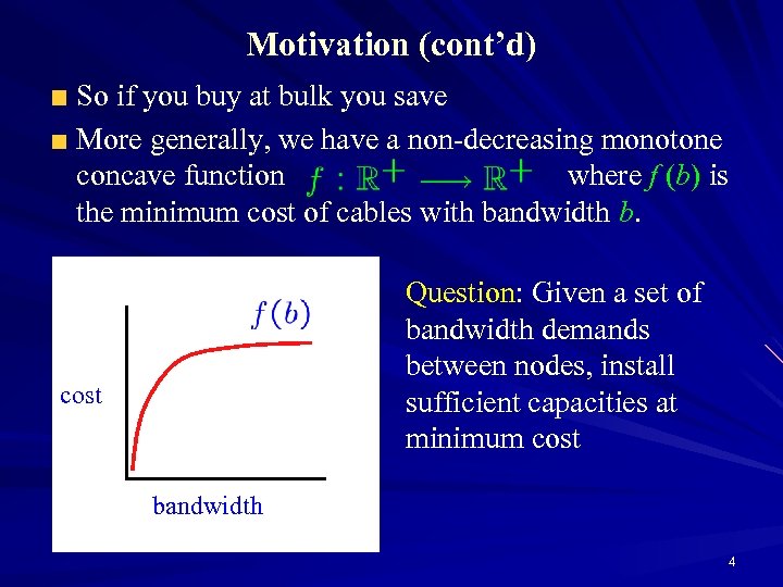
Motivation (cont’d) So if you buy at bulk you save More generally, we have a non-decreasing monotone concave function where f (b) is the minimum cost of cables with bandwidth b. Question: Given a set of bandwidth demands between nodes, install sufficient capacities at minimum cost bandwidth 4

Motivation (cont’d) The previous problem is equivalent to the following problem: There a set of pairs to be connected For each possible cable connection e we can: Buy it at b(e): and have unlimited use Rent it at r(e): and pay for each unit of flow A feasible solution: buy and/or rent some edges to connect every si to ti. Goal: minimize the total cost 5

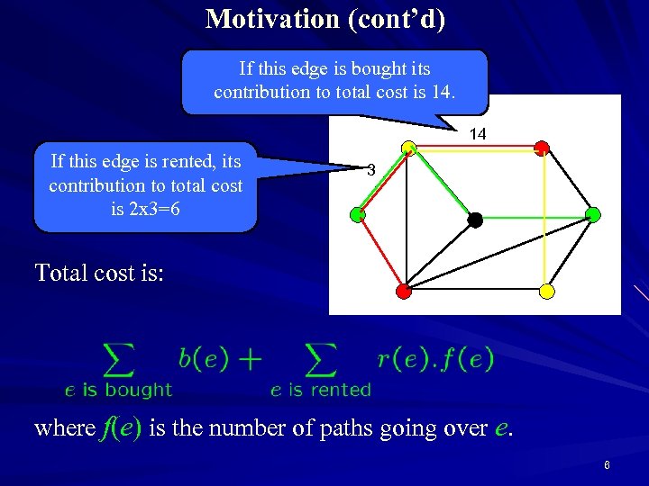
Motivation (cont’d) If this edge is bought its contribution to total cost is 14. 14 If this edge is rented, its contribution to total cost is 2 x 3=6 3 10 Total cost is: where f(e) is the number of paths going over e. 6

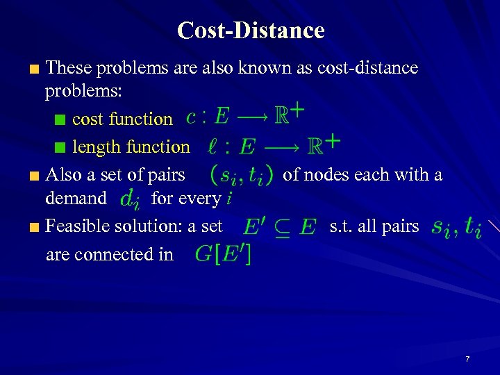
Cost-Distance These problems are also known as cost-distance problems: cost function length function Also a set of pairs of nodes each with a demand for every i Feasible solution: a set s. t. all pairs are connected in 7

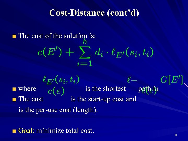
Cost-Distance (cont’d) The cost of the solution is: where is the shortest path in The cost is the start-up cost and is the per-use cost (length). Goal: minimize total cost. 8

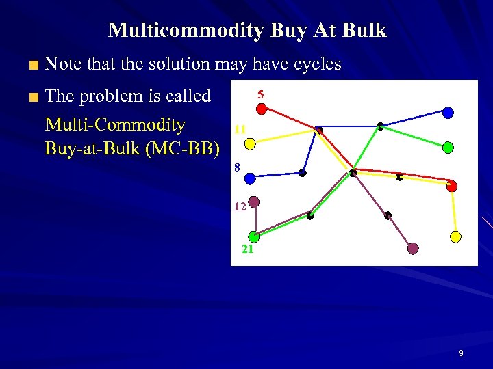
Multicommodity Buy At Bulk Note that the solution may have cycles The problem is called Multi-Commodity Buy-at-Bulk (MC-BB) 5 11 8 12 21 9

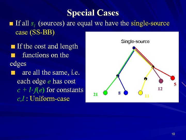
Special Cases If all si (sources) are equal we have the single-source case (SS-BB) If the cost and length functions on the edges are all the same, i. e. each edge e has cost c + l f(e) for constants c, l : Uniform-case Single-source 21 8 12 5 11 10

Previous Work Formally introduced by F. S. Salman, J. Cheriyan, R. Ravi and S. Subramanian, 1997 O(log n) approximation for the uniform case, i. e. each edge e has cost c+l f(e) for some fixed constants c, l (B. Awerbuch and Y. Azar, 1997; Y. Bartal, 1998) O(log n) randomized approximation for the single-sink case: A. Meyerson, K. Munagala and S. Plotkin, 2000 O(log n) deterministic approximation for the single-sink case: C. Chandra, S. Khanna and S. Naor, 2001 11

Hardness Results for Buy-at-Bulk Problems Hardness of Ω(log n) for the singlesink case J. Chuzhoy, A. Gupta, J. Naor and A. Sinha, 2005 Ω(log 1/2 - n) in general Andrews 2004, unless NP ZPTIME(npolylog(n)) 12

Algorithms for Special Cases Steiner Forest A. Agrawal, P. Klein and R. Ravi, 1991 M. X. Goemans and D. P. Williamson, 1995 Single source S. Guha, A. Meyerson and K. Munagala , 2001 K. Talwar, 2002 A. Gupta, A. Kumar and T. Roughgarden, 2002 A. Goel and D. Estrin, 2003 13

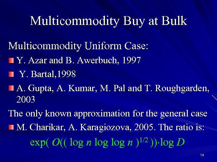
Multicommodity Buy at Bulk Multicommodity Uniform Case: Y. Azar and B. Awerbuch, 1997 Y. Bartal, 1998 A. Gupta, A. Kumar, M. Pal and T. Roughgarden, 2003 The only known approximation for the general case M. Charikar, A. Karagiozova, 2005. The ratio is: exp( O(( log n )1/2 )) log D 14

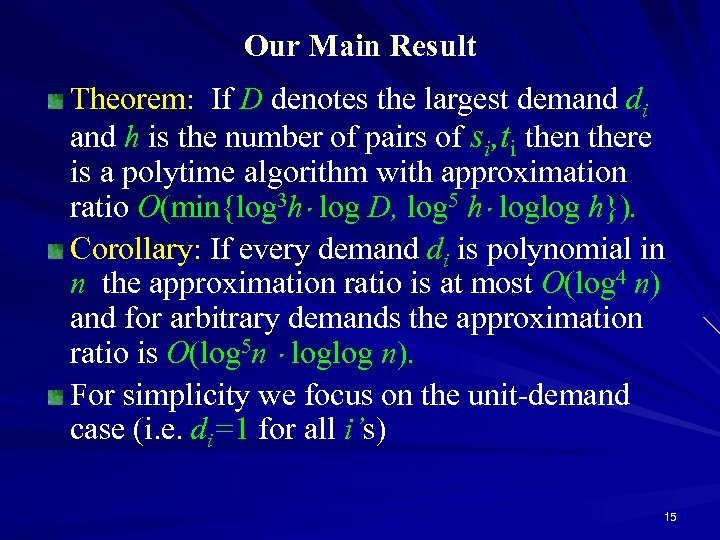
Our Main Result Theorem: If D denotes the largest demand di and h is the number of pairs of si, ti then there is a polytime algorithm with approximation ratio O(min{log 3 h log D, log 5 h loglog h}). Corollary: If every demand di is polynomial in n the approximation ratio is at most O(log 4 n) and for arbitrary demands the approximation ratio is O(log 5 n loglog n). For simplicity we focus on the unit-demand case (i. e. di=1 for all i’s) 15

Recent Development Racke showed how to generalize our junction tree lemma (see later) to exponential demands As a result we can prove: O (log 4 n) - ratio approximation algorithm even if the demands are super-polynomial in n. 16

Overview of the Algorithm The algorithm iteratively finds a partial solution connecting some of the residual pairs The new pairs are then removed from the set; repeat until all pairs are connected (routed) Density of a partial solution = cost of the partial solution # of new pairs routed The algorithm tries to find low density partial solution at each iteration 17

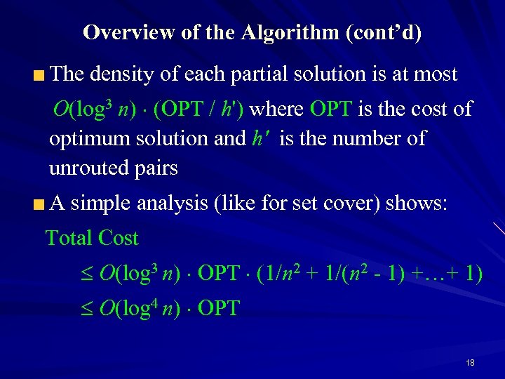
Overview of the Algorithm (cont’d) The density of each partial solution is at most O(log 3 n) (OPT / h') where OPT is the cost of optimum solution and h' is the number of unrouted pairs A simple analysis (like for set cover) shows: Total Cost O(log 3 n) OPT (1/n 2 + 1/(n 2 - 1) +…+ 1) O(log 4 n) OPT 18

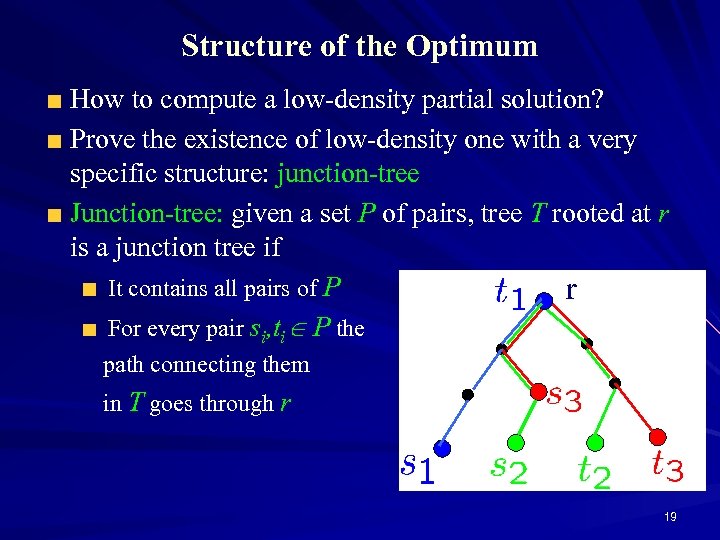
Structure of the Optimum How to compute a low-density partial solution? Prove the existence of low-density one with a very specific structure: junction-tree Junction-tree: given a set P of pairs, tree T rooted at r is a junction tree if It contains all pairs of P r For every pair si, ti P the path connecting them in T goes through r 19

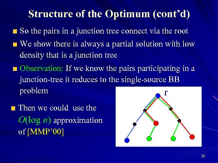
Structure of the Optimum (cont’d) So the pairs in a junction tree connect via the root We show there is always a partial solution with low density that is a junction tree Observation: If we know the pairs participating in a junction-tree it reduces to the single-source BB problem r Then we could use the O(log n) approximation of [MMP’ 00] 20

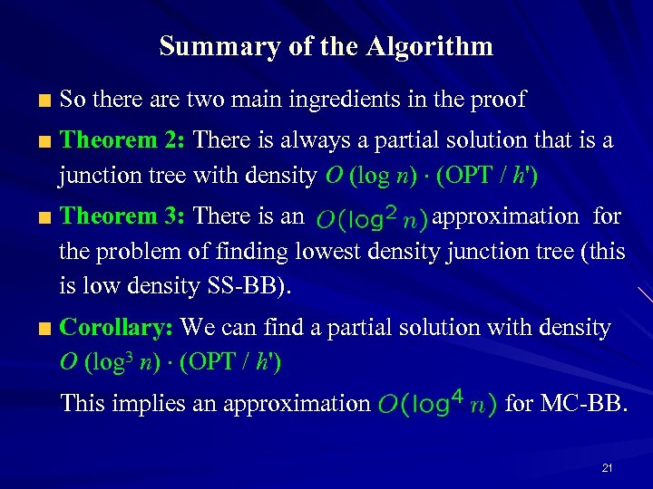
Summary of the Algorithm So there are two main ingredients in the proof Theorem 2: There is always a partial solution that is a junction tree with density O (log n) (OPT / h') Theorem 3: There is an approximation for the problem of finding lowest density junction tree (this is low density SS-BB). Corollary: We can find a partial solution with density O (log 3 n) (OPT / h') This implies an approximation for MC-BB. 21

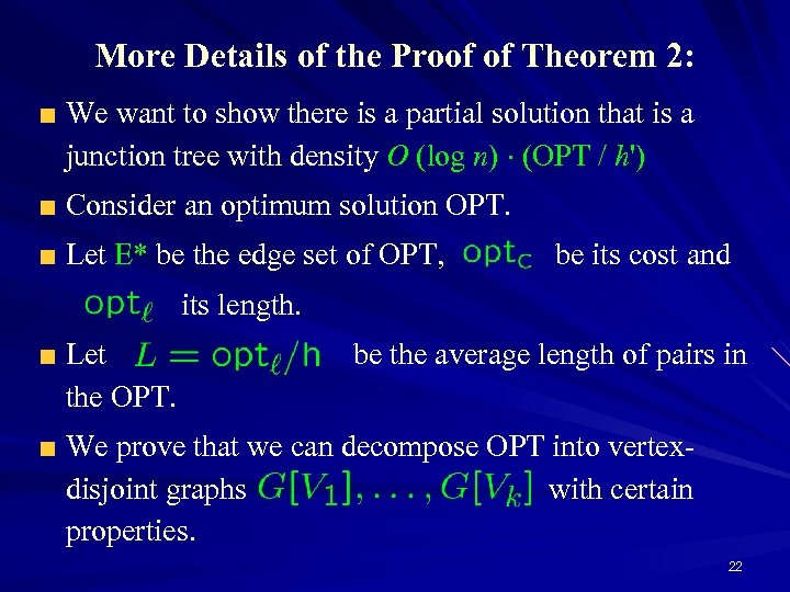
More Details of the Proof of Theorem 2: We want to show there is a partial solution that is a junction tree with density O (log n) (OPT / h') Consider an optimum solution OPT. Let E* be the edge set of OPT, be its cost and its length. Let the OPT. be the average length of pairs in We prove that we can decompose OPT into vertexdisjoint graphs with certain properties. 22

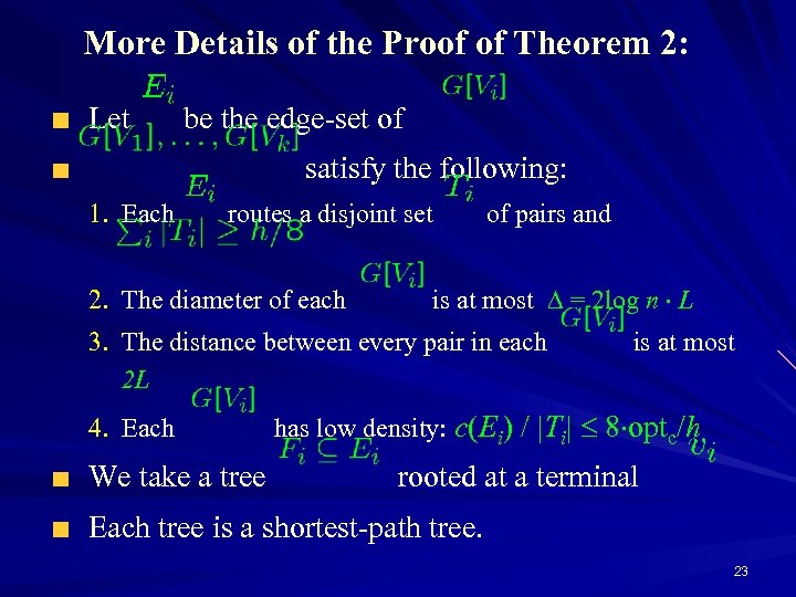
More Details of the Proof of Theorem 2: Let be the edge-set of satisfy the following: 1. Each routes a disjoint set 2. The diameter of each of pairs and is at most = 2 log n L 3. The distance between every pair in each 2 L 4. Each We take a tree is at most has low density: c(Ei) / |Ti| 8 optc/h rooted at a terminal Each tree is a shortest-path tree. 23

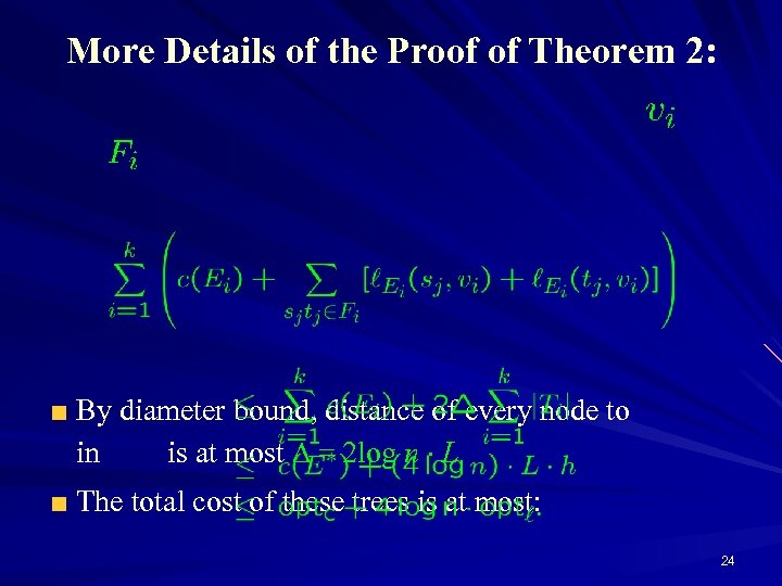
More Details of the Proof of Theorem 2: By diameter bound, distance of every node to in is at most = 2 log n L The total cost of these trees is at most: 24

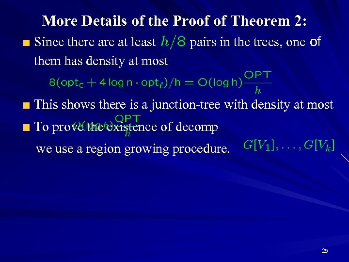
More Details of the Proof of Theorem 2: Since there at least them has density at most pairs in the trees, one of This shows there is a junction-tree with density at most To prove the existence of decomp we use a region growing procedure. 25

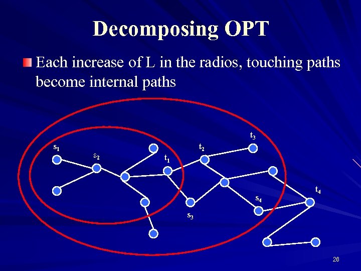
Decomposing OPT Each increase of L in the radios, touching paths become internal paths s 1 s 2 t 1 t 3 s 4 t 4 s 3 26

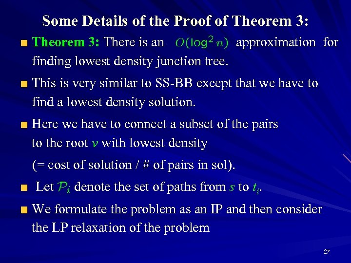
Some Details of the Proof of Theorem 3: There is an approximation for finding lowest density junction tree. This is very similar to SS-BB except that we have to find a lowest density solution. Here we have to connect a subset of the pairs to the root v with lowest density (= cost of solution / # of pairs in sol). Let denote the set of paths from s to ti. We formulate the problem as an IP and then consider the LP relaxation of the problem 27

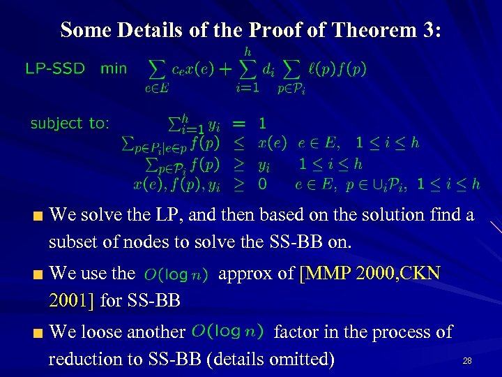
Some Details of the Proof of Theorem 3: We solve the LP, and then based on the solution find a subset of nodes to solve the SS-BB on. We use the 2001] for SS-BB approx of [MMP 2000, CKN We loose another factor in the process of reduction to SS-BB (details omitted) 28

Some Remarks: For the polynomially bounded demand case we can find low density junction-trees using a greedy algorithm The greedy algorithm is based on an algorithm for the k shallow-light tree problem For arbitrary demands, we use the upper bound of M. Elkin, Y. Emek, D. Spielman, S. Teng, (2005) (which is O (log 2 n loglog n)) for distortion in embedding a graph metric into a probability distribution over its spanning trees. 29

Some Remarks (cont’d): This is why we get a factor of for approximation factor comparing to O (log 5 n loglog n)) for polynomially bounded demands. There is a conjectured upper bound of for distortion in embedding a graph metric into a probability distribution over its spanning tree (N. Alon, R. Karp, D. Peleg and D. West, 1991) If true, that would improve our approximation factor for arbitrary demands to 30

Recent Developments Racke: junction trees for exponential demands We use it to get O (log 4 n) ratio for the general case Also, O (log 4 n) ratio approximation for the case of vertex costs Work in progress: O (log 3 n) ratio approximation for MC-BB for polynomial demands 31

Related Problem Given a graph with vertex costs vertex profits and budget B bound, find a maximum profit subtree of budget at most B First algorithm: Guha, Moss, Rabani and Schieber. 2 B cost, opt/O(log 2 n) profit Improvement: Moss and Rabani. 2 B cost, opt/O(log n) profit Kortsarz, Nutov. B budget, opt/(O (log n )) profit Not approximable within loglog n/4 Can handle adding lengths and bounding diameter 32

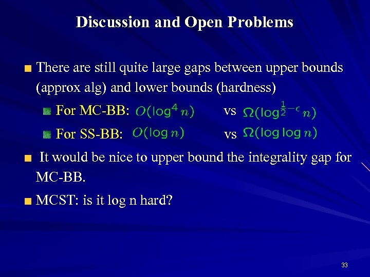
Discussion and Open Problems There are still quite large gaps between upper bounds (approx alg) and lower bounds (hardness) For MC-BB: vs For SS-BB: vs It would be nice to upper bound the integrality gap for MC-BB. MCST: is it log n hard? 33