42c8a2d5239146ae340864a93c32b4d7.ppt
- Количество слайдов: 17

Approximation Algorithms: Bristol Summer School 2008 Seffi Naor Computer Science Dept. Technion Haifa, Israel

Outline 1. Basics 2. Network design – the primal-dual method 3. Network design – iterative rounding and iterative relaxation 4. Competitive analysis via the primal-dial method

Outline 1. Basics 2. Network design – the primal-dual method 3. Network design – iterative rounding and iterative relaxation 4. Competitive analysis via the primal-dial method.
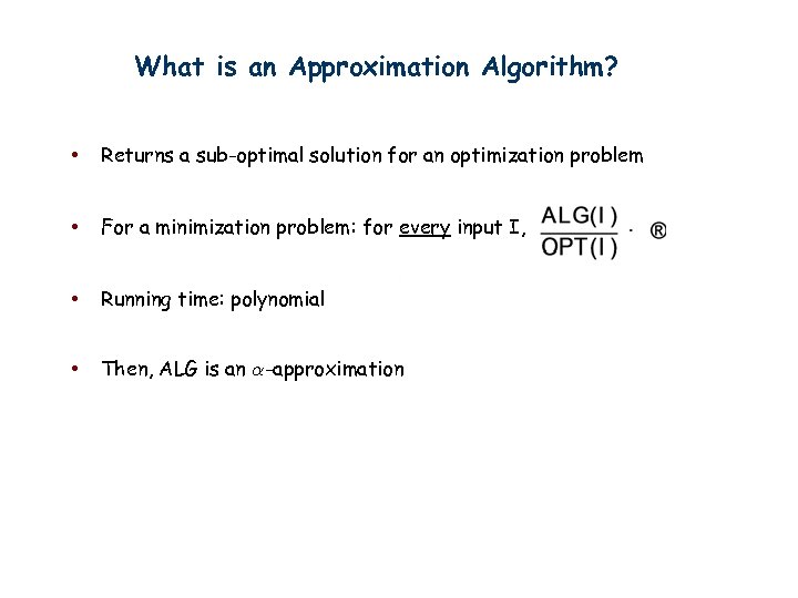
What is an Approximation Algorithm? • Returns a sub-optimal solution for an optimization problem • For a minimization problem: for every input I, • Running time: polynomial • Then, ALG is an ®-approximation
Why are Approximation Algorithms needed? • Many interesting/useful optimization problems are NP-hard • Optimal solution cannot be computed • How well can they be approximated? • Leads to beautiful algorithmic theory. • And, the problems still need to be solved in practice …
Simple Example: Vertex Cover • Input: undirected graph G=(V, E) • Output: a minimum cardinality V’ µ V such that V’ Å e ; for each e 2 E Classic NP-hard problem • Approximation Algorithm: • Find a maximal (inclusion-wise) matching M • Vertex Cover V’ = V(M) , vertices adjacent to edges in M
Analysis Feasibility of cover: V(M) covers all edges, • Every edge must have an end point in V(M) • Otherwise, M is not a maximal matching! Approximation factor: • Optimal solution must pick a representative from each edge e 2 M • Therefore, OPT ¸ V(M)/2 • Approximation factor = V(M)/OPT · 2 Question: Can this factor be improved? Probably not …
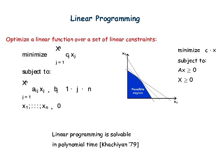
Linear Programming Optimize a linear function over a set of linear constraints: minimize c ¢ x subject to: Ax ¸ 0 X¸ 0 Linear programming is solvable in polynomial time [Khachiyan ’ 79]
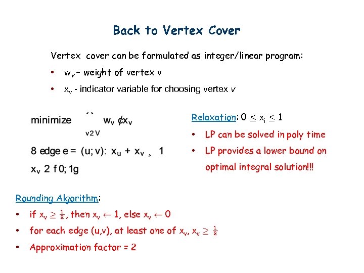
Back to Vertex Cover Vertex cover can be formulated as integer/linear program: • wv – weight of vertex v • xv - indicator variable for choosing vertex v Relaxation: 0 · xi · 1 • LP can be solved in poly time • LP provides a lower bound on optimal integral solution!!! Rounding Algorithm: • if xv ¸ ½, then xv à 1, else xv à 0 • for each edge (u, v), at least one of xv, xu ¸ ½ • Approximation factor = 2
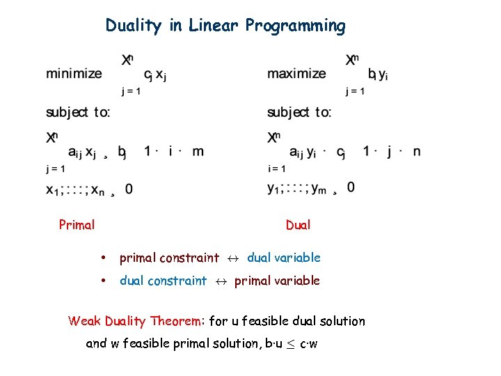
Duality in Linear Programming Primal Dual • primal constraint $ dual variable • dual constraint $ primal variable Weak Duality Theorem: for u feasible dual solution and w feasible primal solution, b·u · c·w
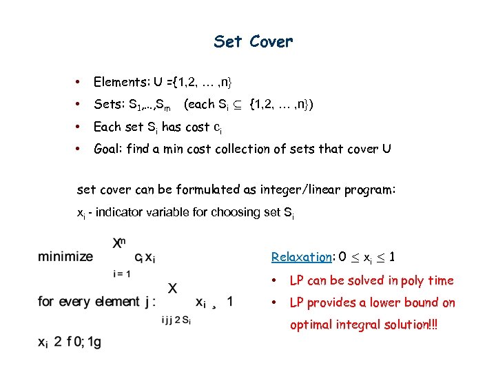
Set Cover • Elements: U ={1, 2, … , n} • Sets: S 1, …, Sm • Each set Si has cost ci • Goal: find a min cost collection of sets that cover U (each Si µ {1, 2, … , n}) set cover can be formulated as integer/linear program: xi - indicator variable for choosing set Si Relaxation: 0 · xi · 1 • LP can be solved in poly time • LP provides a lower bound on optimal integral solution!!!
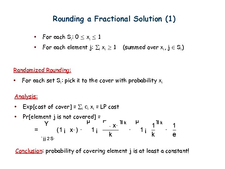
Rounding a Fractional Solution (1) • For each Si: 0 · xi · 1 • For each element j: i xi ¸ 1 (summed over xi, j 2 Si) Randomized Rounding: • For each set Si: pick it to the cover with probability xi Analysis: • Exp[cost of cover] = i ci xi = LP cost • Pr[element j is not covered] = Conclusion: probability of covering element j is at least a constant!
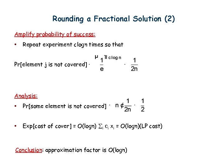
Rounding a Fractional Solution (2) Amplify probability of success: • Repeat experiment clogn times so that Pr[element j is not covered] Analysis: • Pr[some element is not covered] • Exp[cost of cover] = O(logn) i ci xi = O(logn)(LP cost) Conclusion: approximation factor is O(logn)
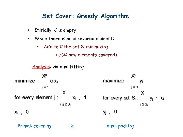
Set Cover: Greedy Algorithm • Initially: C is empty • While there is an uncovered element: • Add to C the set Si minimizing ci/(# new elements covered) Analysis: via dual fitting Primal: covering ¸ dual: packing
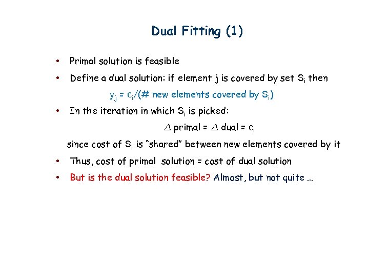
Dual Fitting (1) • Primal solution is feasible • Define a dual solution: if element j is covered by set Si then yj = ci/(# new elements covered by Si) • In the iteration in which Si is picked: ¢ primal = ¢ dual = ci since cost of Si is “shared” between new elements covered by it • Thus, cost of primal solution = cost of dual solution • But is the dual solution feasible? Almost, but not quite …
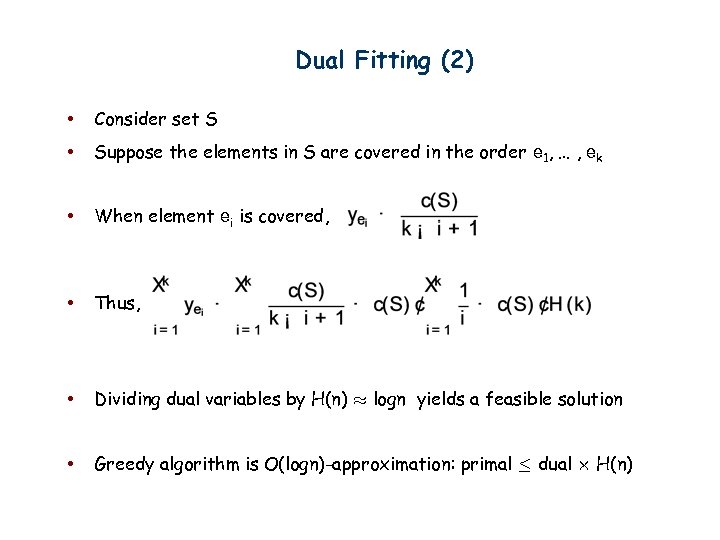
Dual Fitting (2) • Consider set S • Suppose the elements in S are covered in the order e 1, … , ek • When element ei is covered, • Thus, • Dividing dual variables by H(n) ¼ logn yields a feasible solution • Greedy algorithm is O(logn)-approximation: primal · dual £ H(n)
Summary • Linear programming: useful method for relaxing combinatorial problems • Randomized rounding: going from a fractional solution to an integral solution without incurring too much damage • Dual programs: • useful for generating lower bounds • useful for analyzing “primal” algorithms
42c8a2d5239146ae340864a93c32b4d7.ppt