6e5f0a39b6dc51b64a7574b8753bda2c.ppt
- Количество слайдов: 102


Approximate Nearest Neighbor Applications to Vision & Matching Lior Shoval Rafi Haddad

Approximate Nearest Neighbor Applications to Vision & Matching Object matching in 3 D 1. n Recognizing cars in cluttered scanned images n A. Frome, D. Huber, R. Kolluri, T. Bulow, and J. Malik Video Google 2. n A Text Retrieval Approach to object Matching in Videos n Sivic, J. and Zisserman, A

Object Matching n Input: n n Output: n n An object and a dataset of models The most “similar” model Two methods will be presented 1. 2. Object Sq Voting based method Cost based method Model S 1 Model S 2 … Model Sn

A descriptor based Object matching -vote for the model that gave the Voting Every descriptor n n n closet descriptor Choose the model with the most votes Problem n Object Sq The hard vote discards the relative distances between descriptors Model S 1 Model S 2 … Model Sn

A descriptor based Object matching - Cost n Compare all object descriptors to all target model descriptors Object Sq Model S 1 Model S 2 … Model Sn

Application to cars matching

Matching - Nearest Neighbor n n n In order to match the object to the right model a NN algorithm is implemented Every descriptor in the object is compared to all descriptors in the model The operational cost is very high.

Experiment 1 – Model matching

Experiment 2 – Clutter scenes

Matching - Nearest Neighbor n n E. g: Q – 160 descriptors in the object N – 83, 640 [ref. desc. ] X 12 [rotations] ~ 1 E 6 descriptors in the models Exact NN - takes 7. 4 Sec on 2. 2 GHz processor per one object descriptor

Speeding search with LSH n n n Fast search techniques such as LSH (Locality-sensitive hashing) can reduce the search space by order of magnitude Tradeoff between speed and accuracy LSH – Dividing the high dimensional feature space into hypercubes, devided by a set of k randomly-chosen axis parallel hyperplanes & l different sets of hypercubes

LSH – k=4; l=1

LSH – k=4; l=2

LSH – k=4; l=3

LSH - Results n n Taking the best 80/160 descriptors Achieving close results with fewer descriptors

Descriptor based Object matching – Reducing Complexity n Approximate nearest neighbor n Dividing the problem to two stages 1. 2. Preprocessing Querying n Locality-Sensitive Hashing (LSH) n Or. . .

Video Google n A Text Retrieval Approach to object Matching in Videos

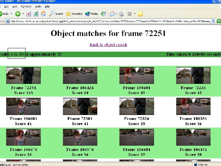
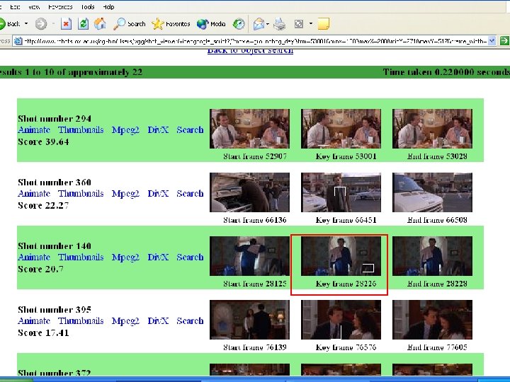
Query Results

Interesting facts on Google The most used search engine in the web

? Who wants to be a Millionaire

How many pages Google search? a. Around half a billion b. Around 4 billions c. Around 10 billions d. Around 50 billions

How many machines do Google use? a. 10 b. Few hundreds c. Few thousands d. Around a million
 Frame/shot 72325 /")
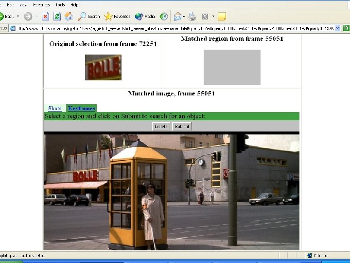
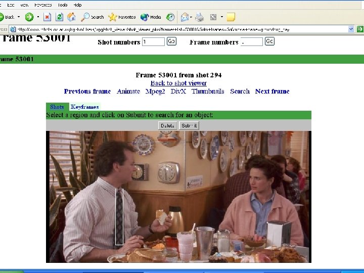
Video Google: On-line Demo Samples Run Lola Run: Supermarket logo (Bolle) Frame/shot 72325 / 824 Red cube logo: Entry frame/shot 15626 / 174 Rolette #20 Frame/shot 94951 / 988 Groundhog Day: Bill Murray's ties Frame/shot 53001/294 Frame/shot 40576/208 Phil's home: Entry frame/shot 34726/172

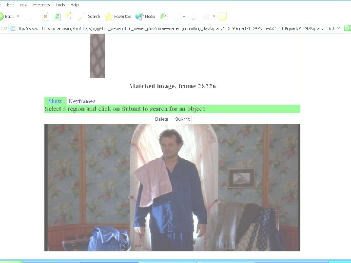
Query
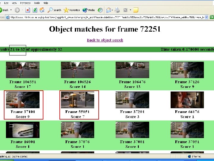

Occluded !!!

Video Google n n n Text Google Analogy from text to video Video Google processes Experimental results Summary and analysis

Text retrieval overview n n n Word & Document Vocabulary Weighting Inverted file Ranking

Words & Documents n n Documents are parsed into words Common words are ignored (the, an, etc) n n Words are represented by their stems n n n This is called ‘stop list’ ‘walk’, ‘walking’, ‘walks’ ’walk’ Each word is assigned a unique identifier A document is represented by a vector n With components given by the frequency of occurrence of the words it contains

Vocabulary n n The vocabulary contains K words Each document is represented by a K components vector of words frequencies (0, 0, … 3, … 4, …. 5, 0, 0)

Example: “…… Representation, detection and learning are the main issues that need to be tackled in designing a visual system for recognizing object. categories ……. ”

Parse and clean represent detect learn Representation, detection and learning are the main issue tackle design main issues that need to be tackled in designing visual system recognize category a visual system for recognizing object categories. …

Creating document vector ID n n Assign unique id to each word Create a document vector of size K with word frequency: n (3, 7, 2, ………)/789 n Or compactly with the original order and position Word Position ID represent 1, 12, 55 1 detect 2, 32, 44, . . . 2 learn 3 3, 11 …… Total …. 789

Weighting n The vector components are weighted in various ways: n n n Naive - Frequency of each word. Binary – 1 if word appear 0 if not. tf-idf - ‘Term Frequency – Inverse Document Frequency’

tf-idf Weighting - Number of occurrences of word i in document - Total number of words in the document - The number of documents in the whole database - The number of occurrences of term i in the whole database => “Word frequency” X “Inverse document frequency” => All documents are equal!

Inverted File – Index Word ID n Crawling stage n n Parsing all documents to create document representing vectors Creating word Indices n An entry for each word in the corpus followed by a list of all documents (and positions in it) 1 2 3 … K Doc. ID 1 2 3 … N

Querying 1. Parsing the query to create query vector Query: “Representation learning” Query Doc ID = (1, 0, 0, …) 2. 3. 4. Retrieve all documents ID containing one of the Query words ID (Using the invert file index) Calculate the distance between the query and document vectors (angle between vectors) Rank the results
 n n n 2. 3. Assume")
Ranking the query results 1. Page Rank (PR) n n n 2. 3. Assume page A has page T 1, T 2…Tn links to it Define C(X) as the number of links in page X d is a weighting factor ( 0≤d≤ 1) Word Order Font size, font type and more

The Visual Analogy Word ? ? ? Stem ? ? ? Document Frame Corpus Film Text Visual

Detecting “Visual Words” “Visual word” Descriptor n n What is a good descriptor? n n n Invariant to different view points, scale, illumination, shift and transformation Local Versus Global How to build such a descriptor ? 1. 2. Finding invariant regions in the frame Representation by a descriptor

Finding invariant regions n Two types of ‘viewpoint covariant regions’, are computed for each frame 1. 2. SA – Shape Adapted MS - Maximally Stable

1. SA – Shape Adapted • • • Finding interest point using Harris corner detector Iteratively determining the ellipse center, scale and shape around the interest point Reference - Baumberg

2. MS - Maximally Stable n n n Intensity water shade image segmentation Iteratively determining the ellipse center, scale and shape Reference - Matas

Why two types of detectors ? n They are complementary representation of a frame n n n SA regions tends to centered at corner like features MS regions correspond to blobs of high contrast (such as dark window on a gray wall) Each detector describes a different “vocabulary” (e. g. the building design and the building specification)

MS - MA example MS – yellow SA - cyan Zoom

Building the Descriptors n SIFT – Scale Invariant Feature Transform n n Each elliptical region is represented by a 128 -dimensional vector [Lowe] SIFT is invariant to a shift of a few pixels (often occurs)

Building the Descriptors n Removing noise – tracking & averaging n n Regions are tracked across sequence of frames using “Constant Velocity Dynamical model” Any region which does not survive for more than three frames is rejected Descriptors throughout the tracks are averaged to improve SNR Large covariance’s descriptors are rejected

The Visual Analogy Word Descriptor Stem ? ? ? Document Frame Corpus Film Text Visual

Building the “Visual Stems” n n n Cluster descriptors into K groups using K-mean clustering algorithm Each cluster represent a “visual word” in the “visual vocabulary” Result: n n 10 K SA clusters 16 K MS clusters

K-Mean Clustering n Minimize square distance of vectors to E. g. Input n A centroidsset of n unlabeled examples D={x 1, x 2, …, xn} in d -dimensional feature space n Number of clusters - K n Objective n Find the partition of D into K non-empty disjoint subsets n So that the points in each subset are coherent according to certain criterion

K-mean clustering - algorithm Step 1: Initialize a partition of D a. Randomly choose K equal size sets and calculate their centers m 1 D={a, b, …, k, l) ; n=12 ; K=4 ; d=2

K-mean clustering - algorithm Step 1: Initialize a partition of D b. For other point y, it is put into subset Dj, if xj is the closest center to y among the K centers m 1 D 1={a, c, l} ; D 2={e, g} ; D 3={d, h, i} ; D 4={b, f, k)

K-mean clustering - algorithm Step 2: Repeat till no update a. Compute the mean (mass center) for each cluster Dj, b. For each xi: assign xi to the cluster with the closest center m 1 D 1={a, c, l} ; D 2={e, g} ; D 3={d, h, i} ; D 4={b, f, k)

K-mean algorithm Final result

K-mean clustering - Cons n n Sensitive to selection of initial grouping and metric Sensitive to the order of input vectors The number of clusters, K, must be determined before hand Each attribute has the same weight

K-mean clustering - Resolution n n Run with different grouping and ordering Run for different K values n Problem ? Complexity!

”MS and SA “Visual Words SA MS

The Visual Analogy Word Descriptor Stem Centroid Document Frame Corpus Film Text Visual

Visual “Stop List” n The most frequent visual words that occur in almost all images are suppressed Before stop list After stop list
 Spatial consistency (= Word")
Ranking Frames 1. 2. Distance between vectors (Like in words/Document) Spatial consistency (= Word order in the text)

Visual Google process n Preprocessing: n n Vocabulary building Crawling Frames Creating Stop list Querying n n Building query vector Ranking results

Vocabulary building Subset of 48 shots is selected 10 k frames = 10% of movie Clustering descriptors using k-mean algo. Parameters tuning is done with the ground truth set Regions construction (SA + MS) 10 k frames * 1600 = 1. 6 E 6 regions SIFT descriptors representation Frames tracking 1. 6 E 6 ~200 k regions Rejecting unstable regions

Crawling Implementation n complexity – per • The To reduceselectedof the one keyframe 5 k expressiveness (100 -150 k frames visual vocabulary second is frames) Frames outside the ground truth set contains new n Descriptors are computed for stable regions in object and scenes, and their detected regions each key frame have not been included in forming the clusters n Mean values are computed using two frames each side of the key frame n Vocabulary: Vector quantization – using the nearest neighbor algorithm (found from the ground truth set)
 Frames tracking 5")
Crawling movies summary Key frames selection Regions construction (SA + MS) Frames tracking 5 k frames Nearest neighbored for vector quantization Stop list SIFT descriptors representation Tf-idf weighting Indexing Rejecting unstable regions

“Google like” Query Object Generate query descriptor Use nearest neighbor algo’ to build query vector Use inverse index to find relevant frames Doc vectors are sparse small set Rank results Calculate distance to relevant frames 0. 1 seconds with a Matlab

Experimental results n The experiment was conducted in two stages: n n Scene location Matching Object retrieval

Scene Location matching n Goal n n Evaluate the method by matching scene locations within a closed world of shots (=‘ground truth set’) Tuning the system parameters

Ground truth set n n 164 frames, from 48 shots, were taken at 19 3 D location in the movie ‘Run Lola Run’ (4 -9 frames from each location) There are significant view point changes in the frames for the same location

Ground Truth Set

Location matching n n The entire frame is used as a query region The performance is measured over all 164 frames The correct results were determined by hand Rank calculation
 ; 0 -")
Location matching Rank Nrel N Ri - Ordering quality (0≤Rank≤ 1) ; 0 - best - number of relevant images - the size of the image set (164) - the location of the i-th relevant image (1≤Ri≤N) in the result if all the relevant images are returned first

Location matching - Example – Frame 6 is the current query frame – Frames 13, 17, 29, 135 contain the same scene location Nrel = 5. – The result was: {17, 29, 6, 142, 19, 135, 13, … Frame number 6 13 17 29 Ri Best Rank 3 “ 7 4 1 “ 2 " 135 Total 6 5 19 15

Location matching Best Rank Query Rank

Rank of relevant frames

Frames 61 - 64

Object retrieval n Goal n n Searching for objects throughout the entire movie The object of interest is specified by the user as a sub part of any frame

(Object query results (1 Run Lola Run results

(Object query results (2 • The expressive power of the visual vocabulary The visual word learnt for ‘Lola’ are used unchanged for the ‘groundhog day’ retrieval! Groundhog Day results

(Object query results (2 n Analysis: n n Both the actual frame returned and the ranking are excellent No frames containing the object are missed n n No false negative The highly ranked frames all do contain the object n Good precision

Google Performance Analysis Vs Object macthing n n n n n Q – Number of queried descriptors (~102) M – Number of descriptors per frame (~103) N – Number of key frames per movie (~104) D – Descriptor dimension (128~102) K – Number of “words” in the vocabulary (16 X 103~103) α - ratio of documents that does not contain any of the Q “words” (~. 1) Brute force NN: Cost = QMND ~ 1011 Google: Query Vector quantization + Distance = QKD + KN QKD + Q(αN)~ Sparse 107 + 105 Improvement factor ~ 104 -: - 106

Video Google Summary n n Immediate run-time object retrieval Visual Word and vocabulary analogy Modular frame work Demonstration of the expressive power of the visual vocabulary

Open issues n n n Automatic ways for building the vocabulary are needed Ranking of retrieval results method as Google does Extension to non rigid objects, like faces

Future thoughts n Using this method for higher level analysis of movies n n Finding content of a movie by the “words” it contains Finding the important (e. g. a star) object in a movie Finding the location of unrecognized video frames More ?

$1 Million!!! What is the meaning of the word Google? a. The number 1 E 10 b. Very big data c. The number 1 E 100 d. A simple clean search

Reference 1. Sivic, J. and Zisserman, A. , Video Google: A Text Retrieval Approach to Object Matching in Videos. Proceedings of the International Conference on Computer Vision (2003) 2. Brin and L. Page. The anatomy of a large-scale hypertextual web search engine. In 7 th Int. WWW Conference , 1998. 3. K. Mikolajczyk and C. Schmid. An affine invariant interest point detector. In Proc. ECCV. Springer. Verlag, 2002. 4. A. Frome, D. Huber, R. Kolluri, T. Bulow, and J. Malik. Recognizing Objects in Range Data Using Regional Point Descriptors. To appear in European Conference on Computer Vision , Prague, Czech Republic, 2004 5. D. Lowe. Object recognition from local scale-invariant features. In Proc. ICCV, pages 1150– 1157, 1999. 6. F. Schaffalitzky and A. Zisserman; Automated Location Matching in Movies 7. J. Matas, O. Chum, M. Urban, and T. Pajdla. Robust wide baseline stereo from maximally stable external regions. In Proceedings of the British Machine Vision Conference , pages 384. 393, 2002. n


Parameter tuning n n K – number of clusters for each region type The initial cluster center values Minimum tracking length for stable features The proportion of unstable descriptors to reject, based on their covariance
 n n n Divide the high - dimensional feature space into")
Locality-Sensitive Hashing (LSH) n n n Divide the high - dimensional feature space into hypercubes, by k randomly chosen axis-parallel hyperplanes Each hypercube is a hash bucket The probability that 2 nearby points are separated is reduced by independently choosing l different sets of hyperplanes 2 hyperplanes

ε-nearest-neighbor
 ≤ (1 + ε) d(q, P) • d(q,")
ε-Nearest Neighbor Search • d(q, p) ≤ (1 + ε) d(q, P) • d(q, p) is the distance between p and q in the euclidean space • • • Normalized distance d(q, p) = (Σ (x(i) – y(i))2)(1/2) Epsilon is the maximum allowed 'error' d(q, P) distance of q to the closest point in P Point p is the member of P that is retrieved (or not)

ε-Nearest Neighbor Search n n Also called approximate Nearest Neighbor searching Reports nearest neighbors to the query point (q) with distances possibly greater than the true nearest neighbor distances n n d(q, p) ≤ (1 + ε) d(q, P) Don't worry, the math is on the next slide

ε-Nearest Neighbor Search Goal • • The goal is not to get the exact answer, but a good approximate answer Many applications of nearest neighbor search where an approximate answer is good enough

ε-Nearest Neighbor Search • • What is currently out? Arya and Mount presented an algorithm • Query time • • Pre-processing • • O(n log n) Clarkson improved dependence on ε • • O(exp(d) * ε-d log n) exp(d) * ε-(d-1)/2 Grows exponentially with d

ε-Nearest Neighbor Search • Striking observation • • “Brute Force” algorithm provides a faster query time • Simply computes the distance from the query to every point in P • Analysis: O(dn) Arya and Mount • “… if the dimension is significantly larger than log n (as it for a number of practical instances), there are no approaches we know of that are significantly faster than brute-force search”

High Dimensions • What is the problem? • • • Many applications of nearest neighbor (NN) have a high number of dimensions Current algorithms do not perform much better than brute force linear searches Much work has been done for dimension reduction

Dimension Reduction • Principal Component Analysis • • • Transforms a number of correlated variables into a smaller number of uncorrelated variables Can anyone explain this further? Latent Semantic Indexing • • Used with the document indexing process Looks at the entire document, to see which other documents contain some of the same words

Descriptor based Object matching - Complexity n Finding for each object descriptor, the nearest descriptor in the model, can be a costly operation n n Descriptor dimension ~ 1 E 2 1000 object descriptors 1 E 6 descriptors per model 56 models Brute force nearest neighbor ~1 E 12
6e5f0a39b6dc51b64a7574b8753bda2c.ppt