d77f243c6e728bd0692e9325f1400989.ppt
- Количество слайдов: 159


Applications in Forensic Genetics Science and Statistics Behind Y STR Systems Wisconsin Department of Justice Madison, WI January 4, 2008 John V. Planz, Ph. D. UNT Center for Human Identification

Assessing the Significance of Y STR Data • Characteristics of Y chromosome and loci • Population structure and distribution of Y haplogroups • Forensic applications • Powerplex Y characteristics • Working with haplotype statistics • What about mixtures

Classic View of Y-Chromosome • TDF master gene • patrilinealinheritance • no recombination in NRY • recombination in PAR • junk-rich, gene poor

Characteristics of the Human Y Chromosome • size: ~ 60 Mb • ~ 35 Mb euchromatic (transcribed) • ~ 25 Mb heterochromatic (non-transcribed) • 95% non-recombining (NRY) • 5% X-recombining (2 pseudoautosomal regions at telomeres) • shape: acrocentric - very short p-arm, long q-arm (“Y” name) • rich in different kinds of repetitive DNA sequences • lack of recombination • relatively poor in gene content

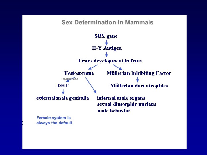
Genes on the Human Y Chromosome • 23 Mb of the euchromatic region determined • 156 transcription units • 78 encode proteins (genes) • 27 distinct Y-specific protein-coding genes (gene families) • 16 ubiquitously expressed genes = housekeeping genes – e. g. RPS 4 Y, ZFY, AMELY, SMCY, DBY • 9 testis-specific genes = male sex determination, spermatogenesis – e. g. SRY, TSPY, CDY, RBMY, DAZ

Genes Mapped to Y Chromosome

Genes on the Human Y Chromosome • 23 Mb of the euchromatic region determined • 156 transcription units • 78 encode proteins (genes) • 27 distinct Y-specific protein-coding genes (gene families) • 16 ubiquitously expressed genes = housekeeping genes • 9 testis-specific genes = male sex determination, spermatogenesis origin of NRY genes: – derived / preserved from the proto-sex chromosomes (X-homology) – specialization in male-specific function

Evolution of Mammalian Sex Chromosomes Lahn, Pearson & Jegalian 2001 Some homology with X – need to consider in validation

Polymorphisms of the Human Y Chromosome Mutations create DNA polymorphisms and these may serve as genetic markers • Single-Copy DNA – e. g. , SNPs, indels • Repetitive DNA – e. g. , STRs
 characterized F > 300 microsatellites")
Y Chromosome Polymorphisms F ~ 200 binary polymorphisms (Y-SNPs) characterized F > 300 microsatellites (Y-STRs) characterized F 1 minisatellite (MSY 1)

Not all mutations occur at the same rate ‘hotspots’ ‘coldspots ’

Mutation Process for STR loci

Y-STR consensus structure and allele ranges

Y-STR consensus structure and allele ranges

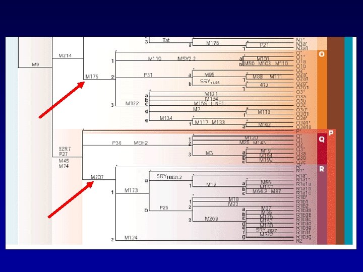
Phylogenetic tree based in binary SNP data
 Forensic Sci. Rev. 15: 91")
Forensic Y STR Systems -From J. M. Butler (2003) Forensic Sci. Rev. 15: 91 -111

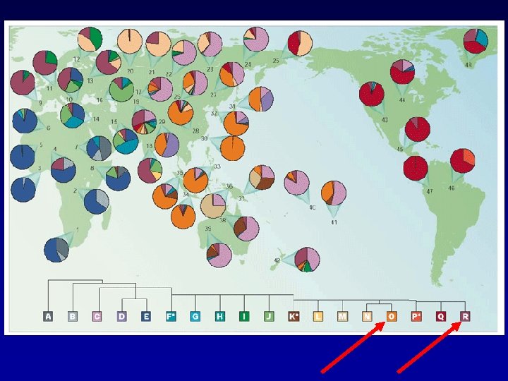
Definitions • Haplotype: combination of allelic states of a set of polymorphic markers lying on the same DNA molecule. • Haplogroup: set of haplotypes defined by slowly mutating markers (mainly SNPs) which have more phylogenetic stability. Unique event polymorphisms (UEP) record history of Y chromosome

Why are our Y haplotypes so different? • Many markers to choose from • The selected loci are physically linked • Markers have both SNPs and STRs Infinite Sites Model Stepwise Mutation Model Infinite Alleles Model

Population Differentiation • Effective population size of Y chromosome is 1/4 of autosomes or 1/3 of X – lower sequence diversity on Y – more susceptible to genetic drift • random changes in frequency of haplotypes due to sampling bias from one generation to next • accelerates differences between populations • Variance of offspring further reduces Ne (effective population size)

Population Differentiation • Geographical clustering due to patrilocal behavior of men – women move closer to man’s birthplace – local geographical differentiation enhanced – Conquest effect From Zerjal et al. Am. J. Hum. Genet. 72: 717– 721, 2003

Population Differentiation • Geographical clustering due to patrilocal behavior of men – women move closer to man’s birthplace – local geographical differentiation enhanced – Conquest effect You must consider that we are not talking about contemporary populations when discussing this! Converse seen with mt. DNA in Native American Populations

Forensic Y-STR Applications – Detect male DNA in a sample containing male and female DNA (Huge background of female DNA) – Aspermic males – Fingernail Scrapings – Additional Power of Discrimination – Multiple male donors – Limits of differential extraction/ tissues – Gender clarification (amelogenin)

A Forensic Application Finger Nail Scraping Case • Victim was found strangled to death • Suspect had scratches on his face • Based on STR results, suspect could not be excluded; many alleles were below interpretation threshold (inconclusive result)

Evidentiary Profile Suspect Profile

Identification of Male Contributor DNA in Crime Scene Material Autosomal STR profile Y STR profile Female Victim DNA: Male Suspect DNA: Large Female DNA: Perpetrator Male DNA - See only female DNA profile - Or partial DNA profile - no female DNA - no profile overlap - only male component

Investigations regarding Paternal Lineages • Paternity Testing • Kinship Analysis • Deficiency cases • Mass disasters • Missing Persons • Unidentified Remains

Deficiency Case Male Lineage ? • Y STR analysis - any male relative in pedigree can be a reference for alleged father

**Remember paternal lineage issues for identity testing

Y-STR Haplotype Analysis in Deficiency Paternity Case ? DYS 19 DYS 389 II DYS 390 DYS 391 DYS 392 DYS 393 DYS 385 DYS 413 YCAII Nephew 14 13 30(16) 25 11 13 12 11 -14 22 -22 3 -7 Son 14 12 29 (16) 24 10 15 12 11 -14 22 -22 3 -7 Exclusion If true biological nephew, then alleged father is excluded as father of child in question Kayser et al. Progress in Forensic Genetics (1998), 7: 494 -496

• For effective use, guidelines are needed • ISFG Recommendations • Combine with existing recommendations (NRC II Report) • Nomenclature, Allelic Ladders, Population Genetics, Statistical Issues

Basic Interpretation Guidelines • Similar to autosomal STRs • Thresholds for detection and interpretation • Stutter • Mixtures – what constitutes a mixture • Validation studies in concert with guidelines • Interpret evidence before knowns

Y STR LOCI • DYS 19 • DYS 398 II • DYS 390 • DYS 391 • DYS 392 • DYS 393 • DYS 385 I/II “Minimal Haplotype” – defined for research only

Y STR Loci DYS 389 – two loci DYS 385 – two loci DYS 19 DYS 389 II DYS 390 DYS 391 DYS 392 DYS 393 DYS 438 DYS 439 DYS 385 a/b SWGDAM
 Marker DYS 385 a/b R primer a b F primer Duplicated regions")
Multi-Copy (Duplicated) Marker DYS 385 a/b R primer a b F primer Duplicated regions are 40, 775 bp apart and facing away from each other DYS 389 I/II II F primer I a=b a b Single Region but Two PCR Products (because forward primers bind twice) DYS 389 II F primer R primer Figure 9. 5, J. M. Butler (2005) Forensic DNA Typing, 2 nd Edition © 2005 Elsevier Academic Press

Kits • Commercially available Y-STR multiplex kits --- allow for standard markers and QA/QC • Most have EMH and SWGDAM recommended loci • Extra loci added to enhance discrimination

Power. Plex® Y System DYS 19 DYS 389 II DYS 390 DYS 391 DYS 392 DYS 393 DYS 437 DYS 438 DYS 439 DYS 385 a/b

Powerplex® Y Allelic ladder 92 alleles

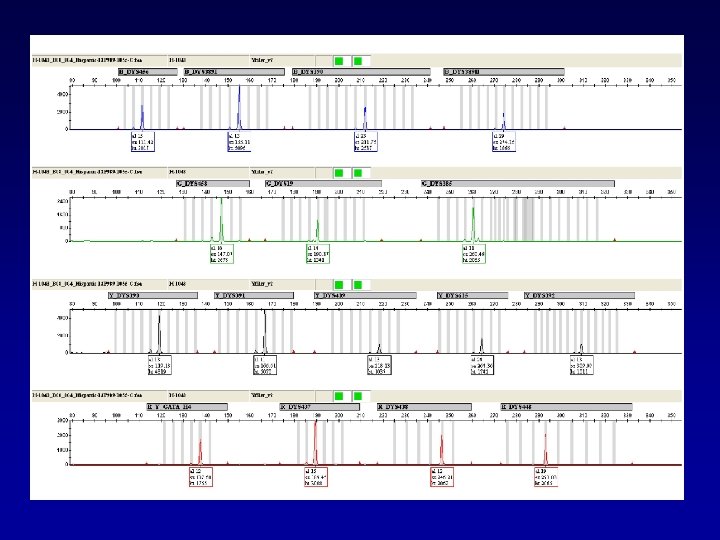
Powerplex® Y Kit 1 ng Male DNA DYS 391 DYS 389 I DYS 438 DYS 439 DYS 437 DYS 393 DYS 389 II DYS 19 DYS 390 DYS 392 DYS 385

Amp. F STR® Yfiler™ Kit DYS 19 DYS 389 II DYS 390 DYS 391 DYS 392 DYS 393 DYS 437 DYS 438 DYS 439 DYS 385 a/b DYS 448 DYS 456 DYS 458 DYS 635 GATA H 4

Amp. F STR® Yfiler™ Allelic ladder 137 alleles

Amp. Fl. STR® Yfiler™ Kit 1 ng Male Control DNA 007 DYS 458 DYS 389 I DYS 390 DYS 389 II DYS 438 DYS 19 DYS 385 a/b DYS 393 Y GATA H 4 DYS 391 DYS 456 DYS 439 DYS 437 DYS 635 DYS 392 DYS 448

What can we expect? Powerplex® Y • Sensitivity • Mixtures • Anomalies

Sensitivity 1. 0 ng 0. 5 ng 0. 25 ng 0. 125 ng 0. 0625 ng 0. 0312 ng

Sensitivity 1. 0 ng 0. 5 ng 0. 25 ng 0. 125 ng 0. 0625 ng 0. 0312 ng

Sensitivity 1. 0 ng 0. 5 ng 0. 25 ng 0. 125 ng 0. 0625 ng 0. 0312 ng

Male-Female Mixture Series 1: 0 1: 1000

Male-Female Mixture Series 1: 0 1: 1000

Male-Female Mixture Series 1: 0 1: 1000

Of course, with Male: Male mixtures you will get more peaks at each locus. Sensitivities down to about 5% minor contributor are typical. You cannot bank on peak height differences to remain consistent across the dyes or loci, so be careful when trying to physically deconvolute these mixtures… this may not be a valid practice! i. e. If target input DNA is 0. 5 ng… 5% minor contributor is only 0. 025 ng

These types of issues should raise some operational questions: F Input DNA: • Total Genomic? • Y specific? • Increase to bring up minor? • Impact of stutter? Valid lab policies and interpretation guidelines must be based on empirical data!

Stutter Issues From Fulmer et al. 2007 Promega Application Notes

DYS 389 II N-1, N-2 stutter is commonly seen at all input template amounts. 1. 0 ng 0. 5 ng 0. 25 ng

1. 0 ng 0. 5 ng 0. 25 ng DYS 392 N-1, N+1 stutter is commonly seen at all input template amounts… this is common among trinucleotide repeat loci.

As with all typing systems, there anomalies that you should be aware of ! The majority of female samples will not produce typing results with the Y STR kits… But remember…the Y and X are functional homologues and recombination IS possible. F always run a female “victim” known when using Y STR kits in the male – female context!

Other observed Powerplex® Y anomalies DYS 19 Primer binding mutation This was in an Asian (Hong Kong) Chinese sample

Other observed Powerplex® Y anomalies “Gene” duplication at DYS 385 a/b R primer a F primer R primer b F primer Multiple mutation steps in the lineage are needed to explain this one!!

Multiband Y Patterns • MN ASIAN PA 0077 DYS 385 - 3 Bands • MN HISPANIC PH 0031 DYS 390 - 2 Bands • MN HISPANIC PH 0063 Multibands • NYC HISPANIC 26 DYS 19 - 2 Bands • NYC CAUCASIAN 4 DYS 19 - 2 Bands • CT HISPANIC 00 -1851 DYS 19 - 2 Bands • CT HISPANIC 99 -1695 DYS 19 - 2 Bands • CT HISPANIC 99 -0362 DYS 19 - 2 Bands • CT HISPANIC 98 -2136 DYS 19 - 2 Bands • CT CAUCASIAN 00 -3022 DYS 385 - 3 Bands • ASIAN A-FTA-34 -F/C DYS 385 - 3 Bands • ASIAN A-FTA-36 -F/C DYS 19 – Primer Binding site? • ASIAN A-FTA-32 -F/C DYS 385 - 4 Bands Must consider this when considering a mixture

Population studies with Powerplex® Y Before we can approach interpretive or statistical understanding of the system we need to understand what we are dealing with as a locus…and yes, the whole set of markers in Powerplex Y are just that…a single locus. Several typical validation issues just don’t matter with a Y haplotype system: • Peak height ratio • Hardy-Weinberg Equilibrium But other things do!

Y STR Population Data Promega Study Population N CFS AFR CT AFR MI AFR NYC AFR TX AFR CFS CAU CT CAU MI CAU NYC CAU TX CAU CT HIS 37 182 86 80 192 57 164 97 83 194 160 MI HIS MN HIS NYC HIS TX HIS Apache Navajo CFS ASN MN ASN NYC ASN TX ASN CFS EI 97 101 80 192 138 219 28 101 45 73 37 Total = 2443
 CFS (n=37) CT (n=182)")
DYS 19 Allele Frequencies African American 0. 5 Sinha (n=543) CFS (n=37) CT (n=182) MI (n=86) NYC (n=80) TX (n=193) 0. 45 0. 4 Frequency 0. 35 0. 3 0. 25 0. 2 0. 15 0. 1 0. 05 0 12 13 14 15 Alleles 16 17 18
/ (n-1) Haplotype Random Match")
Population Parameters Haplotype Diversity h = n(1 - fi 2)/ (n-1) Haplotype Random Match Probability P = fi 2 fi = frequency of each haplotype n = # haplotypes

Y Haplotype Profiles Population N CFS AFR CT AFR MI AFR NYC AFR TX AFR CFS CAU CT CAU MI CAU NYC CAU TX CAU CT HIS MI HIS MN HIS NYC HIS TX HIS 37 182 86 80 193 57 163 97 83 194 158 97 100 80 192 # Haplotypes 36 172 85 80 181 50 153 87 80 170 130 90 95 74 179 % Single Haplotype Diversity 97. 3 94. 5 98. 8 100 93. 8 87. 7 93. 9 89. 7 96. 4 87. 6 82. 3 92. 8 95. 0 92. 5 93. 2 0. 9985 0. 9994 0. 9997 >0. 9999 0. 9993 0. 9944 0. 9991 0. 9968 0. 9991 0. 9981 0. 9963 0. 9985 0. 9988 0. 9968 0. 9991

Y Haplotype Profiles Population Apache Navajo CFS ASN MN ASN NYC ASN TX ASN CFS EI N 138 219 28 100 45 70 37 # Haplotypes 70 101 28 96 43 69 35 % Single Haplotype Diversity 50. 7 46. 1 100 96. 0 95. 6 98. 6 94. 6 0. 9701 0. 9806 >0. 9999 0. 9992 0. 9970 0. 9996 0. 9955

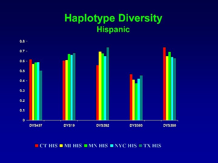
Haplotype Diversity N>80 1. 005 1 0. 995 0. 99 0. 985 0. 98 0. 975 0. 97 0. 965 0. 96 M N A A V SN JO E C H A N IS PA IS TX H A N Y C H H IS IS N M I H IS M T H FR C A TX C A FR FR N Y I A FR M A C C T A U U A TX I C A M C C Y N C T C A U U 0. 955 high haplotype diversity = high intra-individual variation

What about Linkage Equilibrium? Intuitively, since these markers are all on a single chromosome we’d predict strong linkage and a lack of independence between the loci. Although this is very different from what we are used to with our beloved CODIS loci…this is what we expect with a haplotype What do we get?

Y STR Loci Pairwise Tests Population CFS AFR CT AFR MI AFR NYC AFR TX AFR CFS CAU CT CAU MI CAU NYC CAU TX CAU CT HIS MI HIS MN HIS NYC HIS TX HIS 12 Loci – 66 tests N # Equilibrium 37 182 86 80 193 57 163 97 83 194 158 97 100 80 192 35 23 27 34 21 30 26 30 22 11 26 33 42 35 37

Y STR Loci Pairwise Tests 12 Loci – 66 tests Population N Apache Navajo CFS ASN MN ASN NYC ASN TX ASN CFS EI 138 219 28 100 45 70 37 # Equilibrium 9 12 60 50 47 50 35 Fewest – Native American Most – Asian (sample size; but Minnesota and Texas)

Y STR Loci Pairwise Tests 22 populations; ≥ 17 Equilibrium detected Loci 391/389 II 389 I/439 389 I/385 -2 439/389 II 439/393 439/385 -1 439/385 -2 389 II/393 437/393 # Populations 19 18 17 19 18 20 17 18 What’s going on here? ? ? – No detectable linkage?

Y STR Loci Pairwise Tests 22 populations; ≤ 5 Equilibrium Loci 391/438 389 I/389 II 438/437 438/19 438/392 438/385 -1 438/385 -2 437/385 -1 19/392 19/385 -1 392/385 -1 390/385 -1/385 -2 # Populations 5 1 4 4 3 0 4 5 5 3 This is what we’d expect… Strong linkage

Y STR Loci Pairwise Tests 22 Populations – Examples of Population Specific Disequilibrium Loci 389 I/392 438/439 437/385 -2 390/385 -2 # Populations/ Equilibria Population/ Equilibria 15 11 16 12 12 Caucasian African American Likely due to haplogroup differences among populations

What do we see? • There is evidence of “independence” between some of the loci in some of the populations • A combination of mutation rate, subdivision and random drift can cause this. • One of the biggest factors is Haplogroup Diversity • The marker selection for increasing haplotype diversity is not directly correlated to gene diversity.

Approaching Analysis • Some may suggest - “Use the set of Core Y STRs and add more as needed to resolve matches” • First question – when do you stop? • If you get a match, you would have to continue on ad infinitum! • Is this a sensible policy? How much power is needed? ? ?
 Caucasians")
Discriminatory Capacity* for three U. S. populations Y-STR marker combination African American (N=786) Caucasians Hispanics (N=778) (N=381) European minimal haplotype (9) 75. 8% 61. 7% 79. 8% Eur. Minimal + SWGDAM (11) 86. 8% 74. 3% 85. 6% Power. Plex® Y (12) 87. 7% 76. 7% 88. 2% 97. 6% 95. 5% 95. 8% Amp. F STR® Yfiler kit (17) *DC= (# of different haplotypes / pop. size) x 100 Mulero et al. , JFS (2006) 51: 64 -75

Number of Unique Haplotypes Observed for Three U. S. Populations Y-STR marker combination European minimal haplotype (9) African American (N=786) Caucasians (N=778) Hispanics (N=381) 496 382 266 Eur. Minimal + SWGDAM (11) 618 503 295 Power. Plex® Y (12) 628 524 306 749 714 350 Amp. F STR® Yfiler kit (17) Mulero et al. , JFS (2006) 51: 64 -75

Common haplotype identified by the European Minimal Haplotype markers (20 individuals in Yfiler haplotype database*) European Minimal Haplotype # of different haplotypes 0 PP Y Yfiler. TM 8 20 * http: //www. appliedbiosystems. com/yfilerdatabase/

So…the logic does work… More loci… better resolution… But…doesn’t the size of the database matter?
 N= 1000")
# of different haplotypes Individuals sharing haplotypes Point Estimate (N = 3561) N= 1000 European Minimal Haplotype 0 PP® Y Yfiler. TM 6 20 20 4, 4, 2, 6 0 0. 0056 0. 0011 0. 0006 0. 0017 0. 00028 0. 02 0. 004 0. 002 0. 006 0. 001

Approaching Analysis • Unlikely approach because information gain is low • Many samples will already be very limited • Community will rely on commercially available kits not in-house designer systems • QC/ Proficiency Testing • Better to increase size of database(s) to gain power • We will re-visit substructure issues later

Approaching Analysis • Some may suggest - “A reference database should contain related individuals” – to better define the population • Probability of paternal relative having the same haplotype is usually 1 • Databases are typically comprised of unrelated individuals • Although a small unknown number of related individuals may be in a database • Able to address significance of a very closely related profile

Exclusion with 1 mismatch among 12 analyzed Y -STRs Evidence 14 12 28 25 11 13 14, 14 11 15 Known 14 12 28 24 11 13 14, 14 11 15 By having a database of unrelated males one can assess weight of relative (with mutation) versus rarity of haplotype in population

Qualitative Conclusions of Y-STR Haplotype Comparison Exclusion - The two haplotypes are dissimilar; i. e, the reference person is excluded as the contributor of Y-specific DNA of the evidence sample Inclusion/Match - The Y haplotypes from two samples are sufficiently similar and potentially could have originated from the same source, or from a common paternal lineage Inconclusive - Exclusion/Inclusion cannot be definitively inferred due to insufficient data from one or both of the DNA samples

Calculation to Convey to the Court • Frequency estimate not possible • Court desires a frequency estimate • Point Estimate (Counting Method) • Confidence Interval • Approach the same as mt. DNA

Calculation to Convey to the Court • The vast majority of possible haplotypes will not be observed in any database • The counting method is likely to be conservative • A correction for sampling • A correction for substructure ? ?

Calculation to Convey to the Court Approaches • It is more likely that the counting method will be employed by the U. S. laboratories and courts because of its operational simplicity

Limitations of the Counting Method • Non-matched sites of the haplotype are given weight equal to that of different origin (but may have some extra value for substructure) • Mutations are not weighted • Haplotypes of the same paternal lineage can be excluded, when they are subject to mutations • Does not recognize evolutionary changes, and/or effect of convergent mutations
")
For Y haplotype observed, count the number of times the profile is observed (X) p = X/N 95% Upper bound on frequency CI = p ± 1. 96 p(1 -p)/N Where • N is the size of the database

What about for Y haplotype that is not observed in your database? ? The upper bound of the CI is 1 - 1/N Where • is the confidence level (0. 05 for a 95% CI) • N is the size of the database Following: W. E. Ricker, 1937. Journal of the American Statistical Association, Vol. 32, No. 198: 349 -356.

Maximum haplotype frequency • If a Y-haplotype is not seen in a sample of N males then at the level of significance: • Maximum frequency = 1 - 1/N • Confidence level = 1 - • As N becomes larger, maximum frequency becomes closer to point estimate This is why databases will drive our statistical strength
 • 500 3/500 (0. 006)")
Haplotype frequency N frequency • 100 3/100 (0. 03) • 500 3/500 (0. 006) • 1, 000 3/1, 000 (0. 003) • 10, 000 3/10, 000 (0. 0003)

Calculation to Convey to the Court Confidence Interval • In many instances, the evidentiary haplotype may not be observed in the reference database • As a consequence, the usual assumption of a Normal distribution may not apply for Y-STR haplotype frequency estimates • Ricker’s theory (1937) accommodates this requirement • The counts as well as the confidence bounds are divided by the number of haplotypes sampled in the entire database to estimate the probability of a match

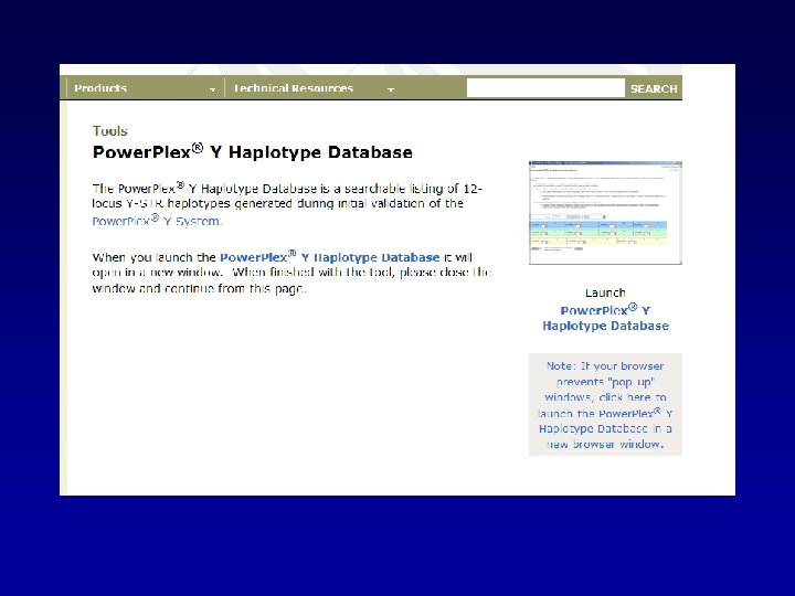
Online available Y-STR haplotype reference databases How de we actually get our Haplotype frequencies? Applied Biosystems Yfiler http: //www. appliedbiosystems. com/yfilerdatabase/ Promega Powerplex Y http: //www. promega. com/techserv/tools/pplexy/default. htm

AB Yfiler

Haplotype data can be input manually or through file upload.

Of Course, There are no matches when testing this many loci.

A random Y haplotype

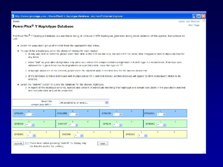
Haplotype data are input manually

Of Course, There are no matches when testing this many loci.

So using our formula from before and an = 0. 05 1 - 1/N 1 – (0. 05)1/4004 = 0. 00075

So, lets try a haplotype that has been seen in the Database…

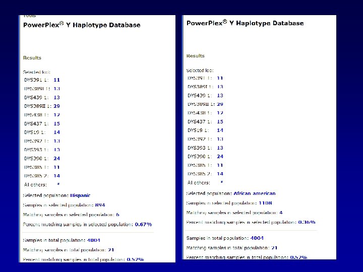
A general search returns 21 matches in the database.
/N What p…? What N…?")
CI = p ± 1. 96 p(1 -p)/N What p…? What N…?

We can evaluate these matches by looking at the distribution of matches among the various population groups.
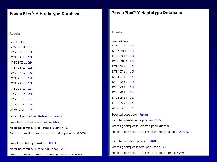

We can do like we did before…looking at the frequency in the whole database: CI = p ± 1. 96 p(1 -p)/N CI = 0. 0052 + 1. 96√ (0. 0052(0. 9948))/4004 Upper bound would be: 0. 00743

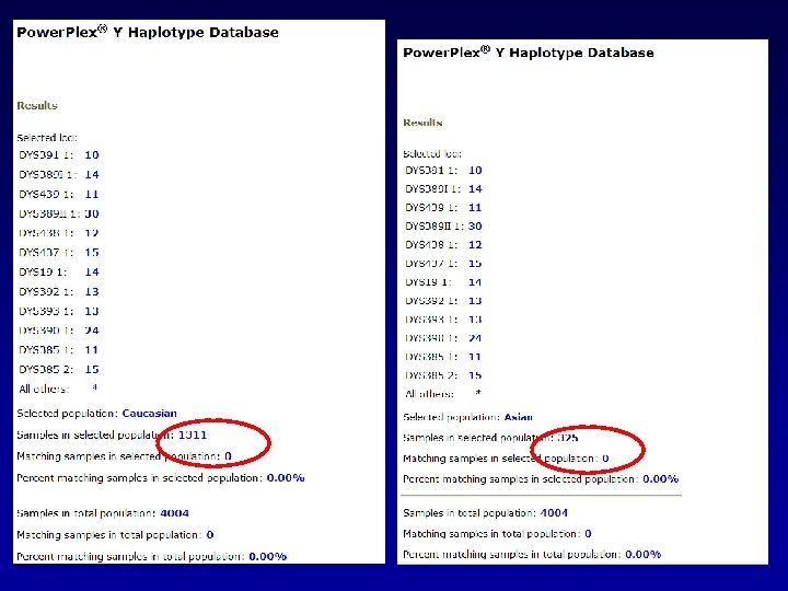
Or we could do specific to the population group in which the match was found: CI = p ± 1. 96 p(1 -p)/N CI = 0. 0076 + 1. 96√ (0. 0076(0. 9924))/1311 Upper bound would be: Caucasians 0. 0123

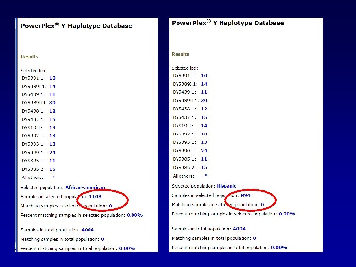
Or we could do specific to the population group in which the match was found: CI = p ± 1. 96 p(1 -p)/N CI = 0. 0067 + 1. 96√ (0. 0067(0. 9933))/894 Upper bound would be: Hispanics 0. 01205

Or we could do specific to the population group in which the match was found: CI = p ± 1. 96 p(1 -p)/N CI = 0. 0036 + 1. 96√ (0. 0036(0. 9964))/1108 Upper bound would be: African American 0. 00712

Calculation to Convey to the Court Population Substructure • Correction for population structure may be considered • Effective population size ¼ of autosomal loci • May actually be a little lower • Substructure effects less in US than ancestral populations • Use when reference database considered not representative

Problems created by population subdivision Haplotype frequencies calculated from population average could lead to: frequencies – Wrong estimates!
 Correction is used as a measure of the effects")
Employ a Theta ( ) Correction is used as a measure of the effects of population substructure (inbreeding, coancestry)

NRCII recommendation was pragmatically set Empirical values are much less for autosomal loci National Academy of Sciences May 1996

Still need to calculate substructure effects But likely to be low for most major populations, if evaluated under a forensic model vs that of an evolutionary model

U. S. Y-STR Haplotype Reference Database www. ystr. org/usa AA CAU HIS Total Number of populations sampled 10 11 9 30 Number of individuals sampled 599 628 478 1, 705 9 9 454 76% 437 70% 354 74% 1116 65% Number of Y-STR loci typed (EMH) Number of different haplotypes Haplotype diversity 99. 8% 99. 6% 99. 5% 99. 7% Most frequent haplotype 12 2. 0% 19 3. 97% 25 3. 98% Kayser et al. J. Forensic Sci. (2002), 47(3): 5513 -519 53 3. 1%

Structure of U. S. Populations with Y-STR Haplotypes Indiana EA Missouri EA Oregon EA Virginia EA European-American Texas EA Cajun EA Lousiana EA Maryland EA New York EA Pennsylvania H Florida EA Connecticut H Hispanic New York H Oregon H Maryland H Lousiana H Texas H Virginia H RST = 0. 1 African-American Lousiana AA Indiana AA Oregon AA Missouri AA Pennsylvania AA New York AA Texas AA Maryland AA Florida AA Virginia AA RST: measure for population differentiation Kayser et al. J. Forensic Sci. (2002), 47(3): 5513 -519
 of genetic variance (AMOVA) Population African American Asian Caucasian Hispanic Native American")
Partition (%) of genetic variance (AMOVA) Population African American Asian Caucasian Hispanic Native American Afr-Cau-His All 5 A 98. 96 98. 69 98. 45 99. 08 96. 98 87. 19 83. 40 B 1. 04 1. 31 1. 55 0. 92 3. 02 1. 25 C -----11. 79 15. 35 A = within sample population B= among sample populations within major population group (or regional variation) C = among major population components for North American populations
 AMOVA routine (with the option of allele size difference) of Arlequin 2.")
FST (AMOVA) AMOVA routine (with the option of allele size difference) of Arlequin 2. 0 Population African American Asian Caucasian Hispanic Native American Afr-Cau-His All 5 FST 0. 0104 0. 0131 0. 0155 0. 0092 0. 0302 0. 1179 0. 1535 ST
 AMOVA routine (without the option of allele size difference) of Arlequin 2.")
FST (AMOVA) AMOVA routine (without the option of allele size difference) of Arlequin 2. 0 Population African American Asian Caucasian Hispanic Native American Afr-Cau-His All 5 ФST 0. 0104 0. 0131 0. 0155 0. 0092 0. 0302 0. 1179 0. 1535 FST 0. 0051 0. 0148 0. 0071 0. 0061 0. 0188 0. 0745 0. 1001 Note: Asian is likely inflated and more data are needed to assess FST
 Population African American Asian Caucasian Hispanic Native American Afr-Cau-His All 5 FST")
FST (AMOVA) Population African American Asian Caucasian Hispanic Native American Afr-Cau-His All 5 FST 0. 0051 0. 0148 0. 0071 0. 0061 0. 0188 0. 0745 0. 1001 FST 0. 0006 0. 0039 -0. 0005 0. 0021 0. 0282 -----autosomal
 = pi + (1 - pi) With of 0. 01 and")
Formula f (haplotype) = pi + (1 - pi) With of 0. 01 and our p of 0. 00028: 0. 00028 + (0. 01 x (1 – 0. 00028)) 0. 00028 + 0. 0099 ≈ 0. 0103 Note: θ is the limiting factor!

Impact Pool populations --- Most frequent • US populations • Intra-individual variation • Most common haplotypes the same • What is the frequency of unknown or uncommon haplotypes in different datasets? • Even if there is substructure

Y STR haplotype is one locus with many alleles Population 1 A 2. . A 100 Databases with reasonable size approximate this model θ is almost 0 A 101 A 102. . A 200 Population 2

Y STR haplotype is one locus with many alleles Population 1 A 2. . An θ approaches 0 A 1' A 2'. . An' Population 2 In reality, with large number of loci a few types are shared and most if not all have never been seen in the database

Y STR haplotype is one locus with many alleles So the more loci typed, the more haplotypes/alleles will be in the database Thus, multi-locus kits are valuable for this aspect approaches 0 In the process of calculating under forensic model***

Forensic Model Population Substructure Which haplotypes might be more closely related? DYS 19 DYS 389 II DYS 390 DYS 391 DYS 392 DYS 393 DYS 385 A --- 14 12 29 24 10 15 12 11 -14 B --- 14 13 29 24 10 15 12 11 -14 C --- 14 13 29 24 12 15 12 10 -14 D --- 18 11 25 24 10 13 15 12 -18 E --- 18 12 25 24 10 15 15 11 -18

Forensic Model Population Substructure Are such evolutionary differences considered in forensic evaluation? DYS 19 DYS 389 II DYS 390 DYS 391 DYS 392 DYS 393 DYS 385 A --- 14 12 29 24 10 15 12 11 -14 C --- 14 13 29 24 12 15 12 10 -14 Exclusion A --- 14 12 29 24 10 15 12 11 -14 E --- 18 12 25 24 10 15 15 11 -18 Exclusion
 Locus Caucasian (N = 199) Afr Amer")
Y STR mutations (father: son allele transmission) Locus Caucasian (N = 199) Afr Amer (N = 203) Hispanic (N = 207) Asian (N = 83) Total (N = 692) DYS 391 11: 10 1 DYS 389 I 12: 13 1 DYS 389 II 29: 30 30: 29 1* DYS 439 13: 12 11: 12 2 DYS 438 0 DYS 437 15: 16 15: 14 2 DYS 19 16: 17 2 17: 16 DYS 392 0 DYS 393 14: 15 1 DYS 390 0 DYS 385 14: 15 12, 14: 14 3 Total 2/2388 6/2436 2/2484 3/996 13/8304 0. 00084 0. 00246 0. 00081 0. 0031 0. 00157
 • 692 confirmed father-son pairs (probability >")
Y STR mutations (father: son allele transmission) • 692 confirmed father-son pairs (probability > 99. 9%) • 14 mutation events were observed • Average rate of 1. 57 x 10 -3/locus /generation (13/8304) • With a 95% confidence bound of 0. 83 x 10 -3 to 2. 69 x 10 -3 • This rate is a little smaller than that of the Kayser, et al. • Estimate (2. 80 x 10 -3/locus) • But the difference is not statistically significant (P > 0. 05). one Asian father-son pair at the DYS 389 I/II loci complex (12, 29) (13, 30) appears as a double mutation, but likely is a single original event.

Paternal Relatives share the same haplotype ? 5 Are they related? Mutation: µ (DYS 393) = 3. 2 x 10 -3 Mutation? ? 7 14, 12, 28, 22, 10, 11, 14 13 -14, 19 -21 f obs= 0. 001 14, 12, 28, 22, 10, 11, 13 13 -14, 19 -21 fobs = 0. 007 Likelihood calculation L(X) = 0. 001 x 5 x µ/2 + 0. 007 x µ/2 (related) L(Y) = 0. 001 x 0. 007 (non-related) LR (X/Y) ≈ 12 for patrilinear relationship

Next Task • Test independence between autosomal loci and Y haplotypes

Independence Testing of Y Haplotype and 13 Autosomal CODIS STR Loci (Autosomal Locus/ Y Haplotype Displaying Disequilibria* - 22 populations) 1. Apache FGA, p‑value = 0. 03760000 D 21 S 11, p‑value = 0. 03460000 D 18 S 51, p‑value = 0. 02820000 D 5 S 818, p‑value = 0. 02660000 2. Minnesota Asian D 8 S 1179, p < 10 -3 3. Minnesota Hispanic D 16 S 539, p‑value = 0. 03340000 D 18 S 51, p‑value = 0. 02100000 4. Canada African American FGA, p‑value = 0. 00920000 5. Canada Asian Indian D 7 S 820, p‑value = 0. 02820000 6. Connecticut African American FGA, p‑value = 0. 04300000 THO 1, p‑value = 0. 00280000 7. Connecticut Caucasian THO 1, p‑value = 0. 02880000 8. Michigan Caucasian D 16 S 539, p‑value = 0. 04820000

Independence Testing of Y Haplotype and 13 Autosomal CODIS STR Loci (Autosomal Locus/ Y Haplotype Displaying Disequilibria* - 22 populations) 9. Michigan Hispanic v. WA, p‑value = 0. 03160000 FGA, p‑value = 0. 02240000 10. Native American Total D 3 S 1358, p‑value = 0. 02680000 D 21 S 11, p‑value = 0. 00060000 D 18 S 51, p‑value = 0. 00840000 11. Navajo D 21 S 11, p‑value = 0. 02820000 12. New York Asian D 16 S 539, p‑value = 0. 00740000 13. New York Caucasian D 7 S 820, p‑value = 0. 01660000 14. New York Hispanic D 21 S 11, p‑value = 0. 01340000 15. Texas African American D 13 S 317, p‑value = 0. 01200000 D 18 S 51, p‑value = 0. 01420000 16. Texas Hispanic D 5 S 818, p‑value = 0. 01880000

Next Task • Mixtures • Assume 2 alleles for 11 loci • 211 possible haplotypes with PP Y – 2048 • Most haplotypes not observed in database • Assumption of independence not correct • Minimal haplotype frequency ( minimum allele frequency) not practical

Mixture • Probability of Exclusion • Binomial distribution - haplotypes excluded and haplotypes not excluded • Count number (m) not excluded; (PI = m/n) • Estimate upper CI of PI • PE = 1 - PI • Based on same principles used for autosomal loci (but at haplotype level)

Mixture Likelihood Ratio • Four scenarios for two contributor sample in example: • Hp --- S 1 and S 2 are source • Hd --- S 1 and unknown are source (same as PI) • Hd --- S 2 and unknown are source (same as PI) • Hd --- two unknowns are source

Mixture Likelihood Ratio • Assume three loci, two alleles at each locus, two male suspects • Total alleles the same as in evidence • Equal contribution • 8 possible haplotypes

PE/PI 13/15 8/10 22/25 --- 3 locus profile All haplotypes included are 13 8 22 --- haplotype 1 15 8 22 --- haplotype 2 13 8 25 --- haplotype 3 15 8 25 --- haplotype 4 13 10 22 --- haplotype 5 15 10 22 --- haplotype 6 13 10 25 --- haplotype 7 15 10 25 --- haplotype 8

PE/PI 13/15, 8/10, 22/25 --- 3 locus profile All possible haplotypes are included 13 8 22 --- haplotype 1 15 8 22 --- haplotype 2 13 8 25 --- haplotype 3 15 8 25 --- haplotype 4 13 10 22 --- haplotype 5 15 10 22 --- haplotype 6 13 10 25 --- haplotype 7 15 10 25 --- haplotype 8 But certain haplotype pairs can not explain evidence haplotype 1 + haplotype 2 haplotype 1 + haplotype 3 haplotype 1 + haplotype 4 haplotype 1 + haplotype 5 and so on

PE/PI 13/15, 8/10, 22/25 --- 3 locus profile All possible haplotypes are included 13 8 22 --- haplotype 1 15 8 22 --- haplotype 2 13 8 25 --- haplotype 3 15 8 25 --- haplotype 4 13 10 22 --- haplotype 5 15 10 22 --- haplotype 6 13 10 25 --- haplotype 7 15 10 25 --- haplotype 8 Only certain haplotype pairs can explain evidence haplotype 1 + haplotype 8 haplotype 2 + haplotype 7 haplotype 3 + haplotype 6 haplotype 4 + haplotype 5
Pr(H 8) + Pr(H 2)Pr(H 7) +")
Mixture Likelihood Ratio 1 LR = 2[Pr(H 1)Pr(H 8) + Pr(H 2)Pr(H 7) + Pr(H 3)Pr(H 6) + Pr(H 4)Pr(H 5)]

Mixture LR • Technically correct • Can not estimate individual haplotype frequencies • 217 (131, 072) possible haplotypes (Yfiler) 211 (2048) possible haplotypes (PP Y) • Not all combinations can explain the evidence • Assuming independence is not correct • Cannot place types in database, most never seen, too many

Use same logic as PI for the denominator in the LR Haplotypes fall into either category E = excluded E = not excluded E/E and E/E pairs can not explain the evidence Only E/E can explain the evidence and only a subset of these fit
 that explain evidence m*/n(n-1) and take")
Mixture LR m* - those pairs (of E/E) that explain evidence m*/n(n-1) and take upper CI as denominator
 • The denominator is the PI with an")
Mixture LR 1 LR = m*/n(n-1) • The denominator is the PI with an assumed number of contributors • Makes better use of data

Online available Y-STR haplotype reference databases Calculation of reporting statistics is quite straight-forward with the help of the searchable databases We still have the problem that none of these (or Pop. Stats) is designed to enable mixture calculations!! And doing this with 12 or 17 loci by hand… …would be a bear!

John V. Planz, Ph. D UNT Center for Human Identification jplanz@hsc. unt. edu

d77f243c6e728bd0692e9325f1400989.ppt