042ce656c903aa4dc79b76d701054471.ppt
- Количество слайдов: 47
Appendix Basic Math for Economics
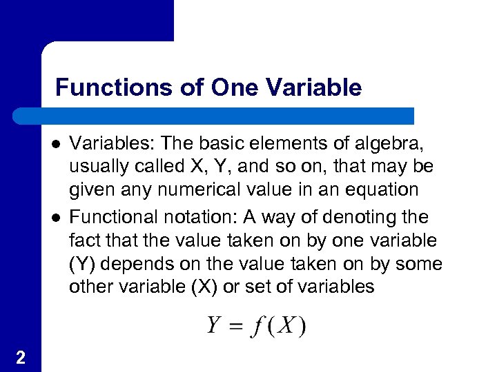
Functions of One Variable l l 2 Variables: The basic elements of algebra, usually called X, Y, and so on, that may be given any numerical value in an equation Functional notation: A way of denoting the fact that the value taken on by one variable (Y) depends on the value taken on by some other variable (X) or set of variables
Independent and Dependent Variables l l 3 Independent Variable: In an algebraic equation, a variable that is unaffected by the action of another variable and may be assigned any value Dependent Variable: In algebra, a variable whose value is determined by another variable or set of variables
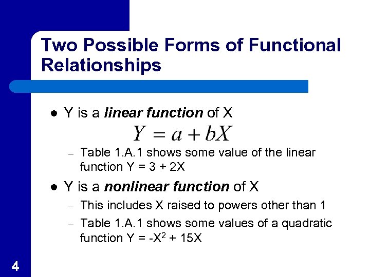
Two Possible Forms of Functional Relationships l Y is a linear function of X – l Y is a nonlinear function of X – – 4 Table 1. A. 1 shows some value of the linear function Y = 3 + 2 X This includes X raised to powers other than 1 Table 1. A. 1 shows some values of a quadratic function Y = -X 2 + 15 X
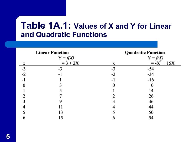
Table 1 A. 1: Values of X and Y for Linear and Quadratic Functions 5
Graphing Functions of One Variable l l Graphs are used to show the relationship between two variables Usually the dependent variable (Y) is shown on the vertical axis and the independent variable (X) is shown on the horizontal axis – 6 However, on supply and demand curves, this approach is reversed
Linear Function l l l 7 A linear function is an equation that is represented by a straight-line graph Figure 1 A. 1 represents the linear function Y=3+2 X As shown in Figure 1 A. 1, linear functions may take on both positive and negative values
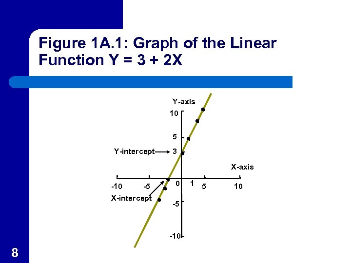
Figure 1 A. 1: Graph of the Linear Function Y = 3 + 2 X Y-axis 10 5 Y-intercept 3 X-axis -10 -5 X-intercept 0 -5 -10 8 1 5 10
Intercept l l The general form of a linear equation is Y = a + b. X The Y-intercept is the value of Y when X equals 0 – 9 Using the general form, when X = 0, Y = a, so this is the intercept of the equation
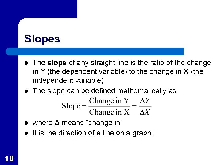
Slopes l l 10 The slope of any straight line is the ratio of the change in Y (the dependent variable) to the change in X (the independent variable) The slope can be defined mathematically as where Δ means “change in” It is the direction of a line on a graph.
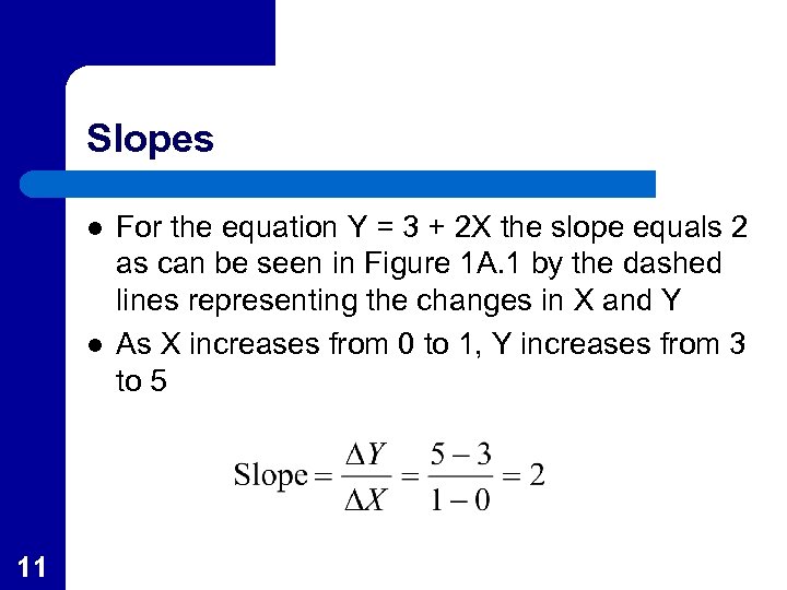
Slopes l l 11 For the equation Y = 3 + 2 X the slope equals 2 as can be seen in Figure 1 A. 1 by the dashed lines representing the changes in X and Y As X increases from 0 to 1, Y increases from 3 to 5
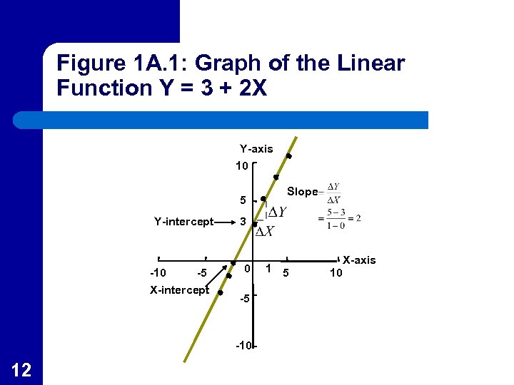
Figure 1 A. 1: Graph of the Linear Function Y = 3 + 2 X Y-axis 10 5 Y-intercept -10 -5 X-intercept 3 0 -5 -10 12 Slope 1 5 X-axis 10
Slopes l l 13 The slope is the same along a straight line. For the general form of the linear equation the slope equals b The slope can be positive (as in Figure 1 A. 1), negative (as in Figure 1 A. 2) or zero If the slope is zero, the straight line is horizontal with Y = intercept

Slope and Units of Measurement l l 14 The slope of a function depends on the units in which X and Y are measured If the independent variable in the equation Y = 3 + 2 X is income and is measured in hundreds of dollars, a $100 increase would result in 2 more units of Y
Slope and Units of Measurement l 15 If the same relationship was modeled but with X measured in single dollars, the equation would be Y = 3 +. 02 X and the slope would equal. 02
Changes in Slope l l l 16 In economics we are often interested in changes in the parameters (a and b of the general linear equation) In Figure 1 A. 2 the (negative) slope is doubled while the intercept is held constant In general, a change in the slope of a function will cause rotation of the function without changing the intercept
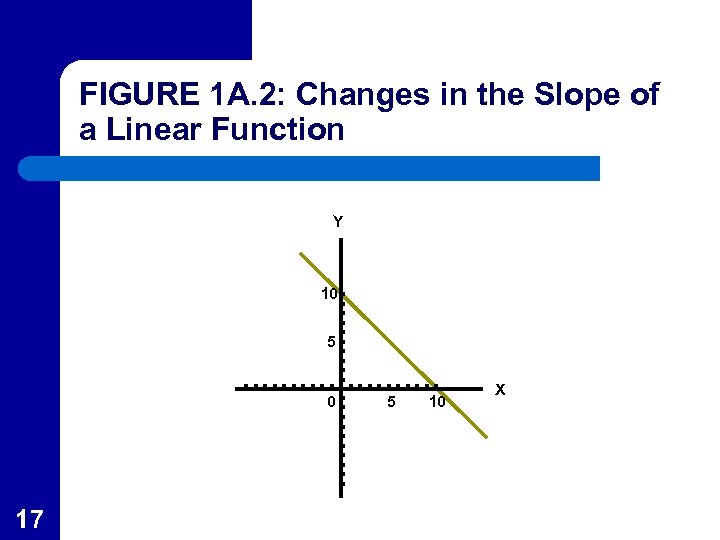
FIGURE 1 A. 2: Changes in the Slope of a Linear Function Y 10 5 0 17 5 10 X

FIGURE 1 A. 2: Changes in the Slope of a Linear Function Y 10 5 0 18 5 10 X
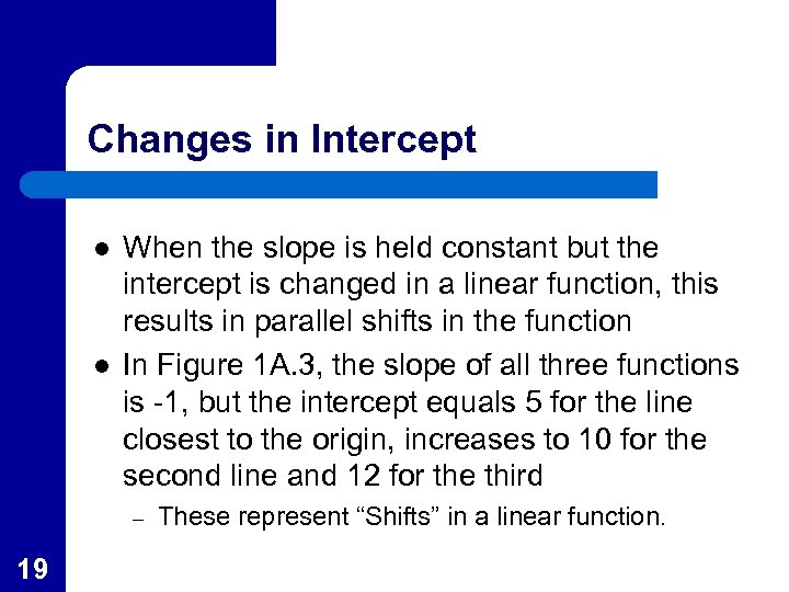
Changes in Intercept l l When the slope is held constant but the intercept is changed in a linear function, this results in parallel shifts in the function In Figure 1 A. 3, the slope of all three functions is -1, but the intercept equals 5 for the line closest to the origin, increases to 10 for the second line and 12 for the third – 19 These represent “Shifts” in a linear function.
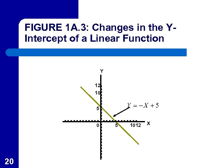
FIGURE 1 A. 3: Changes in the YIntercept of a Linear Function Y 12 10 5 0 20 5 1012 X
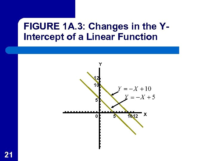
FIGURE 1 A. 3: Changes in the YIntercept of a Linear Function Y 12 10 5 0 21 5 1012 X
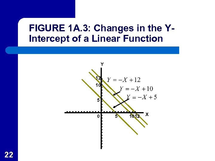
FIGURE 1 A. 3: Changes in the YIntercept of a Linear Function Y 12 10 5 0 22 5 1012 X
Nonlinear Functions l l l 23 Figure 1 A. 4 shows the graph of the nonlinear function Y = -X 2 + 15 X As the graph shows, the slope of the line is not constant but, in this case, diminishes as X increases This results in a concave graph which could reflect the principle of diminishing returns
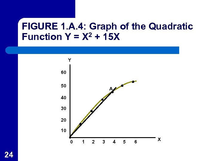
FIGURE 1. A. 4: Graph of the Quadratic Function Y = X 2 + 15 X Y 60 50 A 40 30 20 10 0 24 1 2 3 4 5 6 X
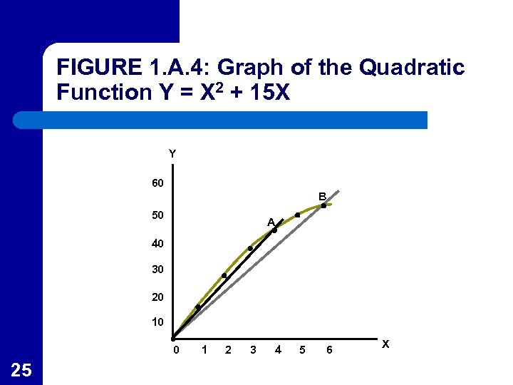
FIGURE 1. A. 4: Graph of the Quadratic Function Y = X 2 + 15 X Y 60 B 50 A 40 30 20 10 0 25 1 2 3 4 5 6 X
The Slope of a Nonlinear Function l l l 26 The graph of a nonlinear function is not a straight line Therefore it does not have the same slope at every point The slope of a nonlinear function at a particular point is defined as the slope of the straight line that is tangent to the function at that point.
Marginal Effects l l 27 The marginal effect is the change in Y brought about by one unit change in X at a particular value of X (Also the slope of the function) For a linear function this will be constant, but for a nonlinear function it will vary from point to point
Average Effects l l 28 The average effect is the ratio of Y to X at a particular value of X (the slope of a ray to a point) In Figure 1 A. 4, the ray that goes through A lies about the ray that goes through B indicating a higher average value at A than at B
APPLICATION 1 A. 1: Property Tax Assessment l l 29 The bottom line in Figure 1 represents the linear function Y = $10, 000 + $50 X, where Y is the sales price of a house and X is its square footage If, other things equal, the same house but with a view is worth $30, 000 more, the top line Y = $40, 000 + $50 X represents this relationship

FIGURE 1: Relationship between the Floor Area of a House and Its Market Value House value (dollars) 160, 000 House without view 110, 000 40, 000 10, 000 0 30 2, 000 3, 000 Floor area (square feet)
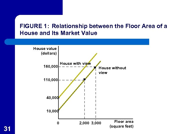
FIGURE 1: Relationship between the Floor Area of a House and Its Market Value House value (dollars) 160, 000 House with view House without view 110, 000 40, 000 10, 000 0 31 2, 000 3, 000 Floor area (square feet)
Calculus and Marginalism l l l 32 In graphical terms, the derivative of a function and its slope are the same concept Both provide a measure of the marginal inpact of X on Y Derivatives provide a convenient way of studying marginal effects.
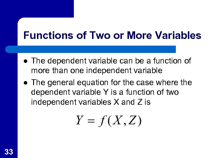
Functions of Two or More Variables l l 33 The dependent variable can be a function of more than one independent variable The general equation for the case where the dependent variable Y is a function of two independent variables X and Z is
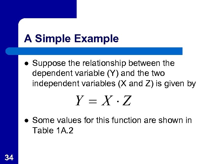
A Simple Example l l 34 Suppose the relationship between the dependent variable (Y) and the two independent variables (X and Z) is given by Some values for this function are shown in Table 1 A. 2
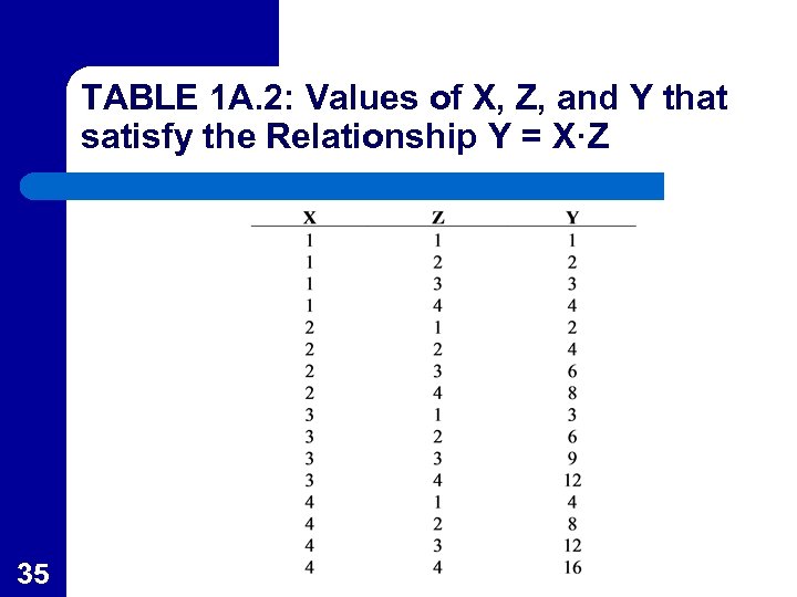
TABLE 1 A. 2: Values of X, Z, and Y that satisfy the Relationship Y = X·Z 35
Graphing Functions of Two Variables l l l 36 Contour lines are frequently used to graph functions with two independent variables Contour lines are lines in two dimensions that show the sets of values of the independent variables that yield the same value for the dependent variable Contour lines for the equation Y = X·Z are shown in Figure 1 A. 5
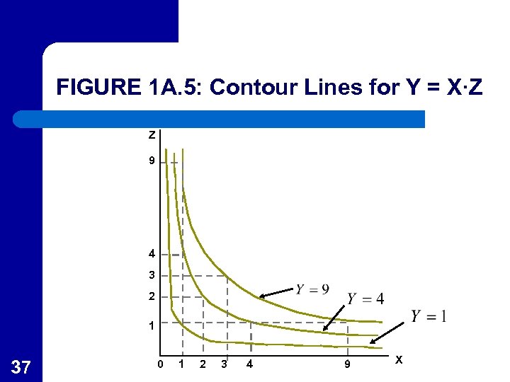
FIGURE 1 A. 5: Contour Lines for Y = X·Z Z 9 4 3 2 1 37 0 1 2 3 4 9 X
Simultaneous Equations l l 38 These are a set of equations with more than one variable that must be solved together for a particular solution When two variables, say X and Y, are related by two different equations, it is sometime possible to solve these equations to get a set of values for X and Y that satisfy both equations
![Simultaneous Equations The equations [1 A. 17] can be solved for the unique solution Simultaneous Equations The equations [1 A. 17] can be solved for the unique solution](https://present5.com/presentation/042ce656c903aa4dc79b76d701054471/image-39.jpg)
Simultaneous Equations The equations [1 A. 17] can be solved for the unique solution 39
![Changing Solutions for Simultaneous Equations The equations [1 A. 19] can be solved for Changing Solutions for Simultaneous Equations The equations [1 A. 19] can be solved for](https://present5.com/presentation/042ce656c903aa4dc79b76d701054471/image-40.jpg)
Changing Solutions for Simultaneous Equations The equations [1 A. 19] can be solved for the unique solution 40
Graphing Simultaneous Equations l l l 41 The two simultaneous equations systems, 1 A. 17 and 1 A. 19 are graphed in Figure 1 A. 6 The intersection of the graphs of the equations show the solutions to the equations systems These graphs are very similar to supply and demand graphs
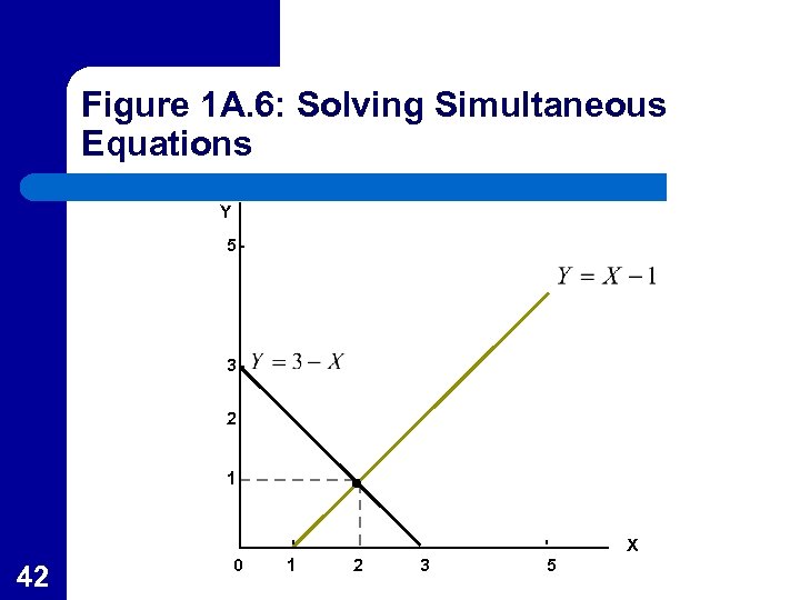
Figure 1 A. 6: Solving Simultaneous Equations Y 5 3 2 1 X 42 0 1 2 3 5
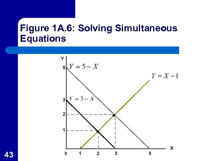
Figure 1 A. 6: Solving Simultaneous Equations Y 5 3 2 1 X 43 0 1 2 3 5
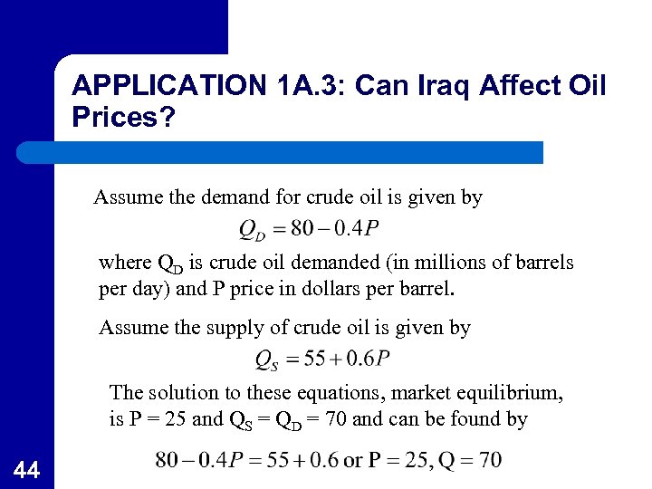
APPLICATION 1 A. 3: Can Iraq Affect Oil Prices? Assume the demand for crude oil is given by where QD is crude oil demanded (in millions of barrels per day) and P price in dollars per barrel. Assume the supply of crude oil is given by The solution to these equations, market equilibrium, is P = 25 and QS = QD = 70 and can be found by 44
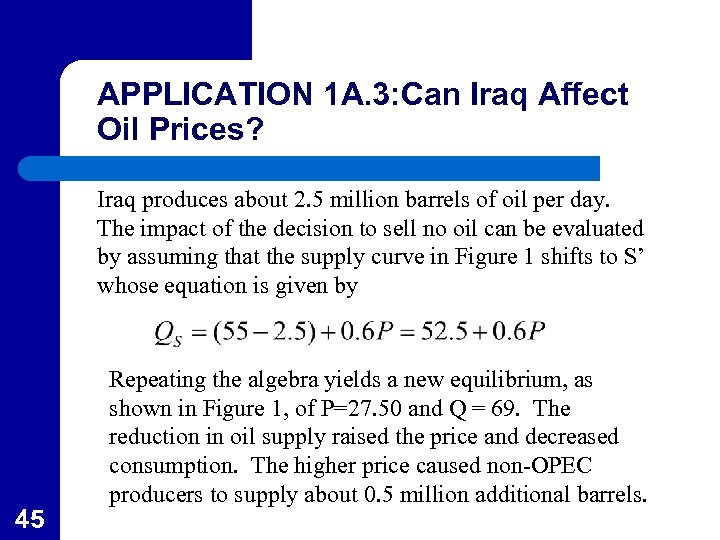
APPLICATION 1 A. 3: Can Iraq Affect Oil Prices? Iraq produces about 2. 5 million barrels of oil per day. The impact of the decision to sell no oil can be evaluated by assuming that the supply curve in Figure 1 shifts to S’ whose equation is given by 45 Repeating the algebra yields a new equilibrium, as shown in Figure 1, of P=27. 50 and Q = 69. The reduction in oil supply raised the price and decreased consumption. The higher price caused non-OPEC producers to supply about 0. 5 million additional barrels.
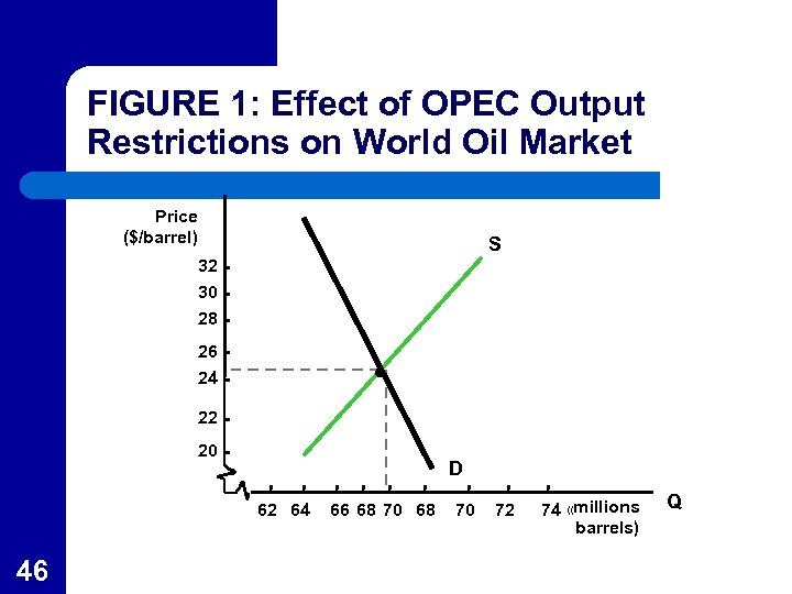
FIGURE 1: Effect of OPEC Output Restrictions on World Oil Market Price ($/barrel) S 32 30 28 26 24 22 20 D 62 64 46 66 68 70 72 74 ((millions barrels) Q
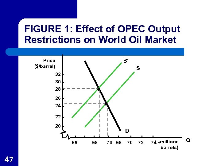
FIGURE 1: Effect of OPEC Output Restrictions on World Oil Market Price ($/barrel) S’ S 32 30 28 26 24 22 20 D 66 47 68 70 72 74 ((millions barrels) Q
042ce656c903aa4dc79b76d701054471.ppt