Anomaly detection using p Trees AKA outlier determination

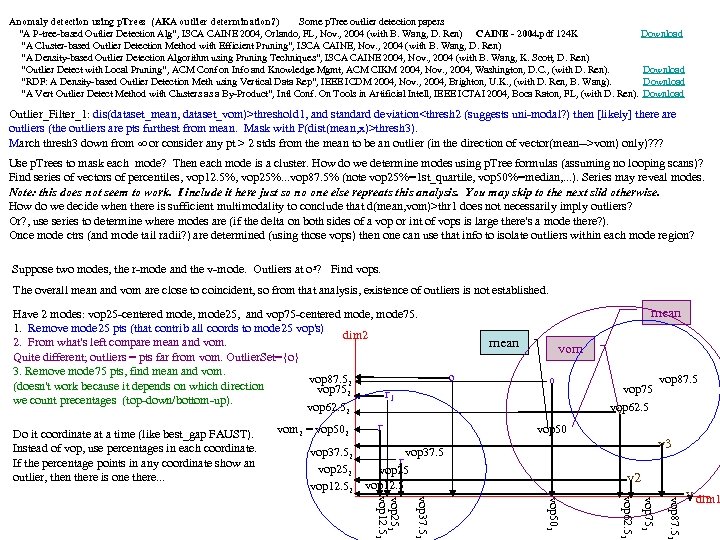Anomaly detection using p. Trees (AKA outlier determination? ) Some p. Tree outlier detection papers “A P-tree-based Outlier Detection Alg”, ISCA CAINE 2004, Orlando, FL, Nov. , 2004 (with B. Wang, D. Ren) CAINE - 2004. pdf 124 K Download “A Cluster-based Outlier Detection Method with Efficient Pruning”, ISCA CAINE, Nov. , 2004 (with B. Wang, D. Ren) “A Density-based Outlier Detection Algorithm using Pruning Techniques”, ISCA CAINE 2004, Nov. , 2004 (with B. Wang, K. Scott, D. Ren) “Outlier Detect with Local Pruning”, ACM Conf on Info and Knowledge Mgmt, ACM CIKM 2004, Nov. , 2004, Washington, D. C. , (with D. Ren). Download “RDF: A Density-based Outlier Detection Meth using Vertical Data Rep”, IEEE ICDM 2004, Nov. , 2004, Brighton, U. K. , (with D. Ren, B. Wang). Download “A Vert Outlier Detect Method with Clusters as a By-Product”, Intl Conf. On Tools in Artificial Intell, IEEE ICTAI 2004, Boca Raton, FL, (with D. Ren). Download Outlier_Filter_1: dis(dataset_mean, dataset_vom)>threshold 1, and standard deviationthresh 3). March thresh 3 down from or consider any pt > 2 stds from the mean to be an outlier (in the direction of vector(mean-->vom) only)? ? ? Use p. Trees to mask each mode? Then each mode is a cluster. How do we determine modes using p. Tree formulas (assuming no looping scans)? Find series of vectors of percentiles, vop 12. 5%, vop 25%. . . vop 87. 5% (note vop 25%=1 st_quartile, vop 50%=median, . . . ). Series may reveal modes. Note: this does not seem to work. I include it here just so no one else repreats this analysis. You may skip to the next slid otherwise. How do we decide when there is sufficient multimodality to conclude that d(mean, vom)>thr 1 does not necessarily imply outliers? Or? , use series to determine where modes are (if the delta on both sides of a vop or int of vops is large there's a mode there? ). Once mode ctrs (and mode tail radii? ) are determined (using those vops) then one can use that info to isolate outliers within each mode region? Suppose two modes, the r-mode and the v-mode. Outliers at o s? Find vops. The overall mean and vom are close to coincident, so from that analysis, existence of outliers is not established. mean Have 2 modes: vop 25 -centered mode, mode 25, and vop 75 -centered mode, mode 75. 1. Remove mode 25 pts (that contrib all coords to mode 25 vop's) dim 2 2. From what's left compare mean and vom. mean vom Quite different; outliers = pts far from vom. Outlier. Set={o} 3. Remove mode 75 pts, find mean and vom. o 0 vop 87. 52 (doesn't work because it depends on which direction vop 752 vop 75 r 1 we count precentages (top-down/bottom-up). vop 62. 52 vop 62. 5 v Do it coordinate at a time (like best_gap FAUST). Instead of vop, use percentages in each coordinate. If the percentage points in any coordinate show an outlier, then there is one there. . . vom 2 = vop 502 vop 37. 52 vop 252 vop 12. 52 vop 87. 51 vop 751 vop 62. 51 vop 501 vop 37. 51 vop 251 vop 12. 51 r vop 50 v 3 vop 37. 5 r vop 25 v 2 vop 12. 5 v dim 1

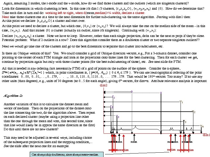Again, assuming 2 modes, the r-mode and the v-mode, how do we find those clusters and the outliers (which are singleton clusters)? Look for dimension in which clustering is best. In this case it's dim 1 (3 clusters, {r 1, r 2, r 3, O}, {v 1, v 2, v 3, v 4} and {0}. How do we determine that? Take each dim in turn and do: working left to right, when d(mean, median)>¼ width, declare a cluster. Next take those clusters one at a time to the next dimension for further sub-clustering via the same algorithm. Starting with dim 1 then: At this point we declare {r 1, r 2, r 3, O} a cluster and start over. At this point we need to declare a cluster, but which one, {0, v 1} or {v 1, v 2}? We will always take the on the median side of the mean - in this case, {v 1, v 2}. And that makes {0} a cluster (actually an outlier, since it's singleton). Continuing with {v 1, v 2}: Declare {v 1, v 2, v 3, v 4} a cluster. Note we have to loop. However, rather than each single projection, delta can be the next m projs if they're close. Potential problem: What if 2 outliers in a row? Does this algorithm consider them as a doubleton cluster or two separate singleton outliers? ? Next we would go take one of the clusters and go to the best dimension to separate that cluster into subclusters, etc. Is there an Oblique version of this? Yes. We could consider a grid of Oblique direction vectors, e. g. , For a 3 -column dataset, consider one pointing to the center of each PTM triangle and look at the projections onto those lines for the best clustering. Then for each cluster we get, continue by projection again but only with those cluster points (for the best subclustering of those), etc. See next slide for PTM. All that is needed is any ordering (not necessarily PTM) of a grid of points on the surface of the sphere. Consider the n-sphere, Sn≡{ x≡(x 1. . . xn) Rn | xi 2=1 } which, in polar coordinates is, { p≡(θ 1. . . θn-1) | 0 θi 179 }. We can use lexicographical ordering of the polar coordinates: 0. . . 00, 0. . . 01, . . . , 0. . . 179, . . . , 10. . . 0, 1110. . . 0, . . . 179. . . 179. That would be 180 n vectors. Too many? If so use any other units (than degrees), e. g. , units of 30 degrees (so 0. . . 5 for each angle), giving 6 n vectors, for dim=n. Attribute relevance analysis is impotant dim 2 Algorithm-2: Another variation of this is to calculate the dataset mean and vector of medians. Then on the projections of the dataset onto the line connecting the two, do the algorithm above. Then repeat on each declared cluster (maybe using a projection line other than the one through the mean and vom, this second time, since that line would likely be in approx the same direction as the first) Do this until there are no new clusters? This may need to be adjusted in several ways, including choice of the subsequent projection lines and the stopping condition, . . . See the slide after the next one for an example. o 0 r 1 v 1 r 2 v 2 r 3 v 4 dim 1 mean median Can always skip doubletons, since always mean=median. mean mean medianmedian

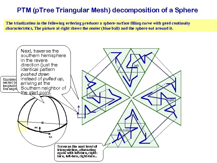PTM (p. Tree Triangular Mesh) decomposition of a Sphere The trixelization in the following ordering produces a sphere-surface filling curve with good continuity characteristics, The picture at right shows the center (blue ball) and the sphere out around it. Next, traverse the Traverse southern hemisphere in the direction (just revere direction (just the identical pattern pushed down instead of pulled up, instead arriving at the Equilateral triangle (90 oof pulled up, sector) bounded by arriving at the Southern neighbor of longitudinal and equatorial Southern neighbor of the start point. line segments the start point. left right dec left turn RA Traverse the next level of triangulation, alternating again with left-turn, rightturn, left-turn, right-turn. .

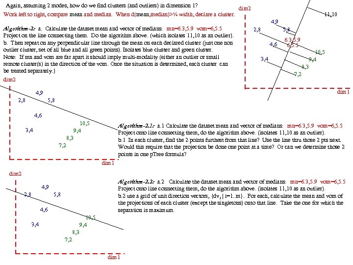Again, assuming 2 modes, how do we find clusters (and outliers) in dimension 1? Work left to right, compare mean and median. When d(mean, median)>¼ width, declare a cluster. Algorithm-2: a. Calculate the dataset mean and vector of medians: mn=6. 3, 5. 9 vom=6, 5. 5 Project on the line connecting them. Do the algorithm above. (which isolates 11, 10 as an outlier). b. Then repeat on any perpendicular line through the mean on each declared cluster (just one non outlier cluster, set of all blue and all green points). Isolates blue cluster and green cluster. Note: If mn and vom are far apart it should imply multi-modality (either an outlier or small remote cluster(s) in the direction of the vom. Once the situation is determined, each cluster can be treated separately. ) dim 2 11, 10 4, 9 2, 8 5, 8 6. 3, 5. 9 4, 6 6, 5. 5 10, 5 3, 4 9, 4 8, 3 7, 2 dim 1 4, 9 2, 8 5, 8 4, 6 10, 5 Algorithm-2. 1: a. 1 Calculate the dataset mean and vector of medians: mn=6. 3, 5. 9 vom=6, 5. 5 3, 4 9, 4 Project onto line connecting them, do the algorithm above. (isolates 11, 10 as an outlier). 8, 3 b. 1 In each cluster, find the 2 points furthest from that line? Use the line thru those 2 pts next. 7, 2 Would this require that the projection be done point at a time? Or can we determine those 2 points in one p. Tree formula? dim 1 dim 2 Algorithm-2. 2: a. 2 Calculate the dataset mean and vector of medians: mn=6. 3, 5. 9 vom=6, 5. 5 4, 9 Project onto line connecting them, do the algorithm above. (isolates 11, 10 as an outlier). 2, 8 5, 8 b. 2 use a grid of unit direction vectors, {dv i | i=1. . m}. For each, calculate the mean and vom of the projections of each cluster (except the singletons) onto that line. Take the one for which the 4, 6 separation is maximum. 10, 5 3, 4 9, 4 8, 3 7, 2 dim 1

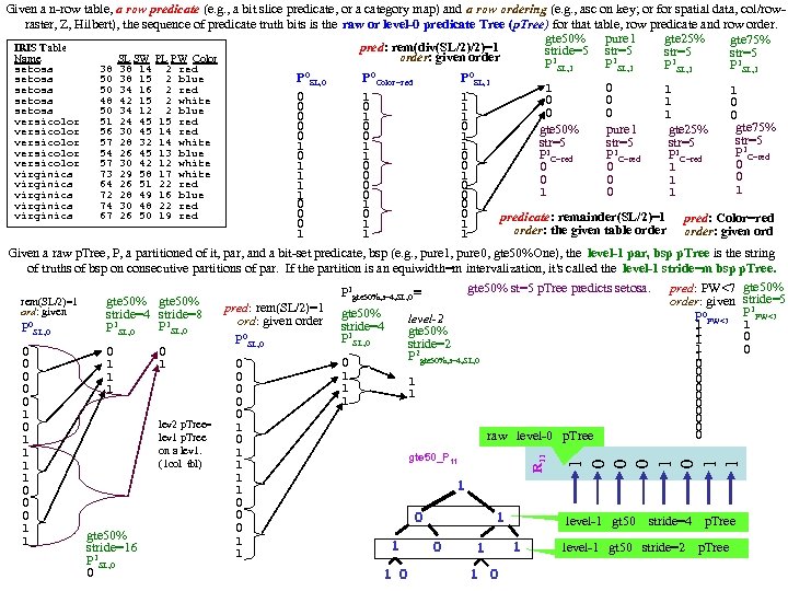
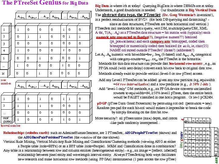The PTree. Set Genius for Big Data is where it's at today! Querying Big. Data is where DBMSs are at today. Underneath, a good foundation is needed. Our foundations is Big Vertical Data The abstract data type, the PTree. Set (Dr. Greg Wettstein's invention!), is a perfect residualization of BVD! (for both DB querying and datamining? - since as data structures, PTree. Sets are both horizontal and vertical. ) PTree. Sets incl methods for horiz query, vert DM, multihop. Query/DM, XML A tbl, T(A 1. . . An) as a PTree. Set data structure = bit matrix with (typically) each numeric attr converted to fixedpt(? ), (negative numers? ? ) bitsliced (pt_pos schema) and each category attr bitmapped; coded then bitmapped or numerically coded then bisliced (or as is, ie, char(25) NAME col stored outside PTree. Set? (dates? ) (addresses? ) Let A 1. . Ak numeric with bitwidths=bw 1. . bwk (0 -based) and Ak+1. . An categorical with category-counts=cc k+1. . . ccn, the PTree. Set is the bitmatrix: Methods for this data structure can provide fast horizontal row access , e. g. , an FPGA could (with zero delay) convert each bit-row back to original data row. . Ak+1, c . . . An, cc 0 1 0 0 1 1 0 0 0 1 0 0 5 0 0 1 0 0 0 1 . . . 1 0 0 0 1 0 0 N 0 0 1 0 0 Methods already exist to provide vertical (level-0 or raw p. Tree) access. Add any Level 1 PTree. Set can be added: given any row partition (eg, equiwidth =64 row intervalization) and a row predicate (e. g. , 50% 1 -bits ). Add "level-1 only" DM methods, e. g. , an FPGA device converts unclassified rowsets to equiwidth=64, 50% level 1 p. Trees, then the entire batch would be FAUST classified in one horiz program. Or lev 1 p. CKNN. A 1, bw . . . A 1, 0 1 1 0 0 2 0 1 3 0 4 -1 1 1 row number 1 n 0 0 1 0 1 1 2 0 1 0 0 0 BPP Relationships (rolodex cards) such as Adenine. Human. Genome, are 2 PTree. Sets, AHGPeople. PTree. Set (shown) and the AHGBase. Pair. Position. PTree. Set (the rotation of the one shown). Vertical Rule Mining, Vertical Multi-hop Rule Mining and Classification/Clustering methods (viewing AHG as either a People table (cols=BPPs) or as a BPP table (cols=People). MRM and Classification done in combination? Any table is a relationship between row and column entities (heterogeneous entity) - e. g. , an image = [reflect. labelled] relationship between pixel entity and wavelength interval entity. Always PTree. Setting both ways facilitates new research and make horizontal row methods (using FPGAs) instantaneous (1 pass across the row p. Tree) AHG(P, bpp) 0 More security? : all p. Trees same (max) depth, and intron -like pads randomly interspersed. . . 5. . . 3 B 0 4 0 3 0 2 0 0 1 0 . . . p. DGP (p. Tree Darn Good Protection) by permuting col ord (permution = key). Random pre-pad for each bit-col would makes it impossible to break the code by simply focusing on the first bit row. 1 0 0 1 1 0 0 0 1 0 0 0 1 1 2 3 4 0 1 n 0 0 0 1 0 1 0 0 1 1 2 5. . . 0 1 A 2, bw 7 B . . . An, cc . . . A 1, 0 -1 1 P Ak+1, c A 1, bw roof 1 (N/64) inteval number 2 . . . A 1, bw 1 A 2, bw

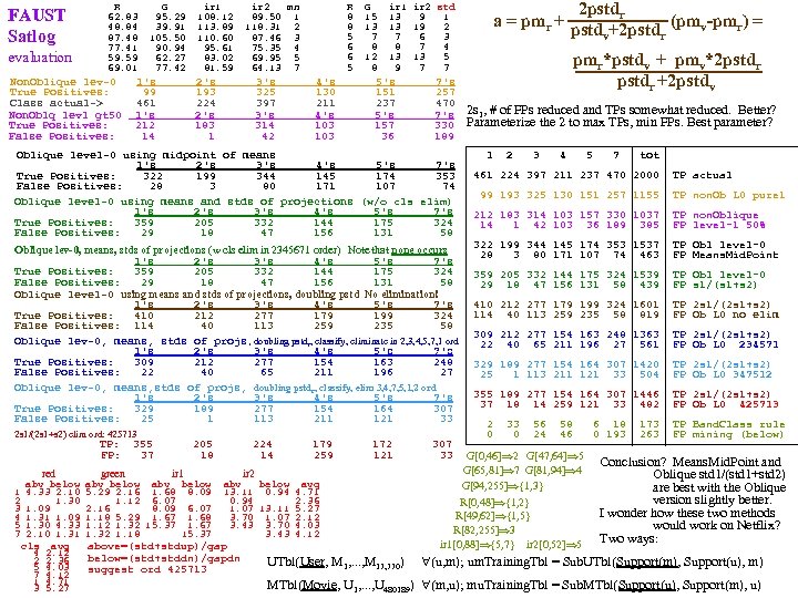
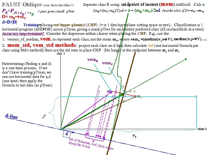FAUST Oblique (our best classifier? ) PR=P(X o d R ) < a 1 pass gives class. R p. Tree R D≡ m. R m. V d=D/|D| Separate class R using midpoint of means (mom) method: Calc a (m. R+(m. V-m. R)/2)od = a = (m. R+m. V)/2 od (works also if D=m. V m. R, Training≡placing cut-hyper-plane(s) (CHP) (= n-1 dim hyperplane cutting space in two). Classification is 1 horizontal program (AND/OR) across p. Trees, giving a mask p. Tree for each entire predicted class (all unclassifieds at-a-time) Accuracy improvement? Consider the dispersion within classes when placing the CHP. E. g. , use the 1. vectors_of_median, vom, to represent each class, not the mean m. V, where vom. V ≡(median{v 1|v V}, median{v 2|v V}, . . . ) 2. mom_std, vom_std methods: project each class on d-line; then calculate std (one horizontal formula per class using Md's method); then use the std ratio to place CHP (No longer at the midpoint between mr and mv dim 2 vom. R Note: training (finding a and d) is a one-time process. If we don’t have training p. Trees, we can use horizontal data for a, d (one time) then apply the formula to test data (as p. Trees) r vv r m. R r v v v r r v m. V v r v v 2 d-line vom. V dim 1 d std of along distances, v the do line d, from ori gin v 1

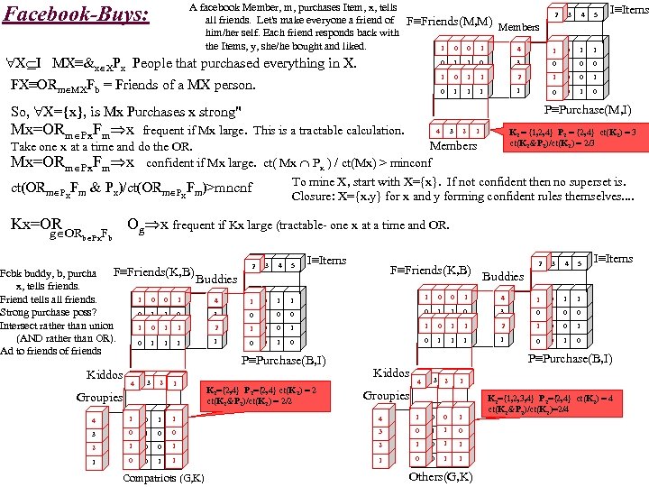
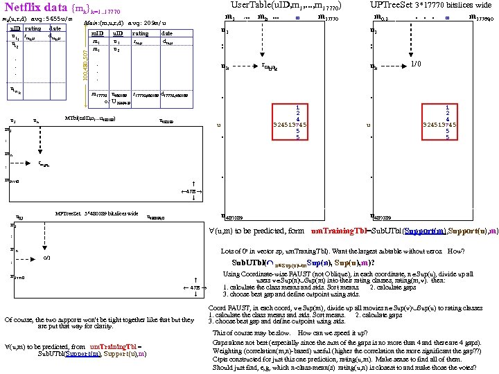
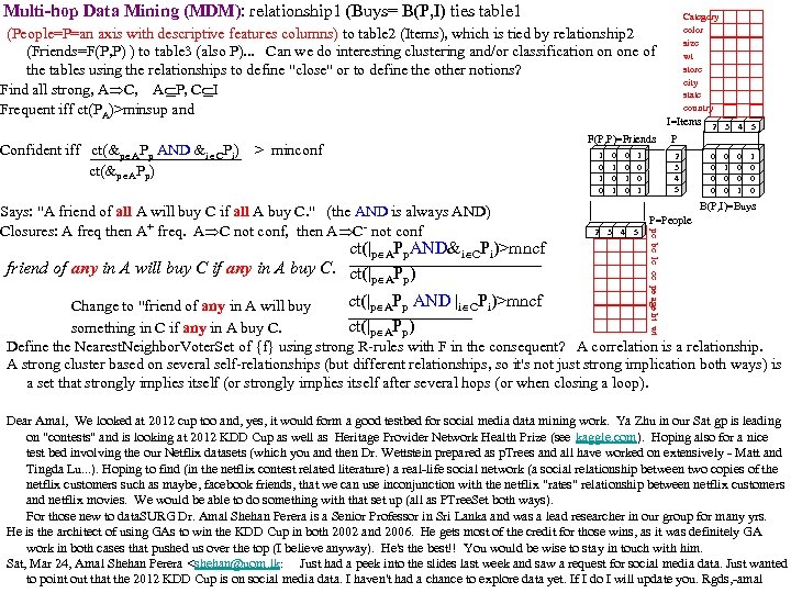Multi-hop Data Mining (MDM): relationship 1 (Buys= B(P, I) ties table 1 (People=P=an axis with descriptive features columns) to table 2 (Items), which is tied by relationship 2 (Friends=F(P, P) ) to table 3 (also P). . . Can we do interesting clustering and/or classification on one of the tables using the relationships to define "close" or to define the other notions? Find all strong, A C, A P, C I Frequent iff ct(PA)>minsup and Confident iff ct(&p APp AND &i CPi) > minconf ct(&p APp) ct(|p APp. AND&i CPi)>mncf friend of any in A will buy C if any in A buy C. ct(| P ) p A p 1 0 1 0 0 1 I=Items 2 3 4 5 0 0 0 0 0 1 1 0 0 0 P 2 3 4 5 B(P, I)=Buys P=People 2 3 4 5 pc bc lc cc pe age ht wt Says: "A friend of all A will buy C if all A buy C. " (the AND is always AND) Closures: A freq then A+ freq. A C not conf, then A C- not conf F(P, P)=Friends Category color size wt store city state country ct(|p APp AND |i CPi)>mncf Change to "friend of any in A will buy ct(|p APp) something in C if any in A buy C. Define the Nearest. Neighbor. Voter. Set of {f} using strong R-rules with F in the consequent? A correlation is a relationship. A strong cluster based on several self-relationships (but different relationships, so it's not just strong implication both ways) is a set that strongly implies itself (or strongly implies itself after several hops (or when closing a loop). Dear Amal, We looked at 2012 cup too and, yes, it would form a good testbed for social media data mining work. Ya Zhu in our Sat gp is leading on "contests" and is looking at 2012 KDD Cup as well as Heritage Provider Network Health Prize (see kaggle. com). Hoping also for a nice test bed involving the our Netflix datasets (which you and then Dr. Wettstein prepared as p. Trees and all have worked on extensively - Matt and Tingda Lu. . . ). Hoping to find (in the netflix contest related literature) a real-life social network (a social relationship between two copies of the netflix customers such as maybe, facebook friends, that we can use inconjunction with the netflix "rates" relationship between netflix customers and netflix movies. We would be able to do something with that set up (all as PTree. Set both ways). For those new to data. SURG Dr. Amal Shehan Perera is a Senior Professor in Sri Lanka and was a lead researcher in our group for many yrs. He is the architect of using GAs to win the KDD Cup in both 2002 and 2006. He gets most of the credit for those wins, as it was definitely GA work in both cases that pushed us over the top (I believe anyway). He's the best!! You would be wise to stay in touch with him. Sat, Mar 24, Amal Shehan Perera

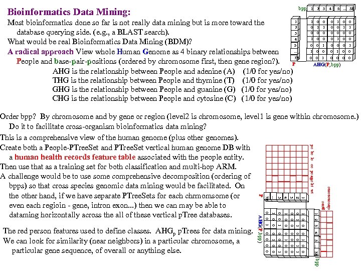bpp Bioinformatics Data Mining: 1 Most bioinformatics done so far is not really data mining but is more toward the 2 database querying side. (e. g. , a BLAST search). 3 4 What would be real Bioinformatics Data Mining (BDM)? 5. . . A radical approach View whole Human Genome as 4 binary relationships between 7 B People and base-pair-positions (ordered by chromosome first, then gene region? ). P AHG is the relationship between People and adenine (A) (1/0 for yes/no) THG is the relationship between People and thymine (T) (1/0 for yes/no) GHG is the relationship between People and guanine (G) (1/0 for yes/no) CHG is the relationship between People and cytosine (C) (1/0 for yes/no) 1 2 3 1 0 0 4 0 1 0 0 0 5 . . . 3 B 1 0 0 0 1 0 0 1 1 0 0 0 0 0 1 0 0 0 AHG(P, bpp) 1 0 1 0 0 1 0 0 2 0 1 0 0 3 0 0 1 0 0 0 0 4 1 0 0 1 5. . . 3 B 1 2 3 4 0 0 5. . . AHG(P, bpp) 0 1 0 0 0 The red person features used to define classes. AHGp p. Trees for data mining. We can look for similarity (near neighbors) in a particular chromosome, a particular gene sequence, of overall or anything else. 7 B P gene chromosome pc bc lc cc pe age ht wt Order bpp? By chromosome and by gene or region (level 2 is chromosome, level 1 is gene within chromosome. ) Do it to facilitate cross-organism bioinformatics data mining? This is a comprehensive view of the human genome (plus other genomes). Create both a People-PTree. Set and PTree. Set vertical human genome DB with a human health records feature table associated with the people entity. Then use that as a training set for both classification and multi-hop ARM. A challenge would be to use some comprehensive decomposition (ordering of bpps) so that cross species genomic data mining would be facilitated. On the other hand, if we have separate PTree. Sets for each chrmomsome (or even each regioin - gene, intron exon. . . ) then we can may be able to dataming horizontally across the all of these vertical p. Tree databases. bpp

A facebook Member, m, purchases Item, x, tells all friends. Let's make everyone a friend of F≡Friends(M, M) Members him/her self. Each friend responds back with the Items, y, she/he bought and liked. 0 1 1 0 1 4 Facebook-Buys: X I MX≡&x XPx People that purchased everything in X. FX≡ORm MXFb = Friends of a MX person. 2 3 4 5 1 0 1 I≡Items 1 0 1 1 0 3 0 1 0 1 1 2 1 0 0 1 1 1 1 0 0 1 0 P≡Purchase(M, I) So, X={x}, is Mx Purchases x strong" Mx=ORm Px. Fm x frequent if Mx large. This is a tractable calculation. 4 3 2 K 2 = {1, 2, 4} P 2 = {2, 4} ct(K 2) = 3 ct(K 2&P 2)/ct(K 2) = 2/3 1 Members Take one x at a time and do the OR. Mx=ORm Px. Fm x confident if Mx large. ct( Mx Px ) / ct(Mx) > minconf To mine X, start with X={x}. If not confident then no superset is. ct(ORm Px. Fm & Px)/ct(ORm Px. Fm)>mncnf Closure: X={x. y} for x and y forming confident rules themselves. . Kx=OR Og x frequent if Kx large (tractable- one x at a time and OR. g ORb Px. Fb F≡Friends(K, B) Fcbk buddy, b, purchases Buddies x, tells friends. 0 1 1 0 1 4 Friend tells all friends. Strong purchase poss? 3 0 1 1 0 Intersect rather than union 1 0 1 1 2 (AND rather than OR). 1 0 1 1 1 Ad to friends of friends Kiddos 4 4 3 2 1 1 Groupies 44 1 1 0 1 4 5 I≡Items 2 3 4 5 4 1 0 3 0 1 0 0 1 2 1 0 0 1 1 1 0 0 1 0 3 1 0 1 1 1 0 1 0 0 0 1 1 1 F≡Friends(K, B) 1 0 0 P≡Purchase(B, I) K 2={2, 4} P 2={2, 4} ct(K 2) = 2 ct(K 2&P 2)/ct(K 2) = 2/2 Buddies P≡Purchase(B, I) Kiddos 4 4 3 2 2 1 1 Groupies 1 1 44 1 1 0 0 0 33 0 0 1 0 0 0 33 22 1 1 0 0 1 1 22 1 1 0 1 1 11 0 0 0 1 1 0 11 0 0 0 1 1 1 0 Compatriots (G, K) I≡Items 1 2 Others(G, K) K 2={1, 2, 3, 4} P 2={2, 4} ct(K 2) = 4 ct(K 2&P 2)/ct(K 2)=2/4

1 0 0 0 1 1 R 11 Given a n-row table, a row predicate (e. g. , a bit slice predicate, or a category map) and a row ordering (e. g. , asc on key; or for spatial data, col/rowraster, Z, Hilbert), the sequence of predicate truth bits is the raw or level-0 predicate Tree (p. Tree) for that table, row predicate and row order. gte 50% pure 1 gte 25% gte 75% pred: rem(div(SL/2)/2)=1 IRIS Table stride=5 str=5 order: given order Name SL SW PL PW Color P 1 SL, 1 setosa 38 38 14 2 red 0 0 0 P SL, 0 P Color=red P SL, 1 setosa 50 38 15 2 blue 1 0 1 setosa 50 34 16 2 red 1 0 1 1 setosa 48 42 15 2 white 0 0 1 0 0 0 1 setosa 50 34 12 2 blue 0 0 1 1 versicolor 51 24 45 15 red 0 0 0 gte 75% gte 50% pure 1 gte 25% versicolor 56 30 45 14 red 0 0 1 str=5 versicolor 57 28 32 14 white str=5 1 1 1 versicolor 54 26 45 13 blue P 1 C=red P C=red 0 1 0 versicolor 57 30 42 12 white 0 1 0 0 1 virginica 73 29 58 17 white 1 0 0 0 1 virginica 64 26 51 22 red 1 0 0 1 1 0 1 virginica 72 28 49 16 blue 1 0 0 0 1 0 virginica 74 30 48 22 red 0 0 0 virginica 67 26 50 19 red predicate: remainder(SL/2)=1 pred: Color=red 0 1 1 order: the given table order: given ord 1 1 1 Given a raw p. Tree, P, a partitioned of it, par, and a bit-set predicate, bsp (e. g. , pure 1, pure 0, gte 50%One), the level-1 par, bsp p. Tree is the string of truths of bsp on consecutive partitions of par. If the partition is an equiwidth=m intervalization, it's called the level-1 stride=m bsp p. Tree. gte 50% st=5 p. Tree predicts setosa. pred: PW<7 gte 50% P 1 gte 50%, s=4, SL, 0 ≡ order: given stride=5 rem(SL/2)=1 gte 50% 1 pred: rem(SL/2)=1 gte 50% ord: given stride=4 stride=8 P 0 PW<7 P PW<7 level-2 ord: given order stride=4 1 1 0 1 1 P SL, 0 gte 50% 1 0 P 1 SL, 0 P 0 SL, 0 1 stride=2 1 0 0 P 2 gte 50%, s=4, SL, 0 1 0 1 0 1 0 1 0 0 0 1 0 lev 2 p. Tree= 0 1 0 0 raw level-0 p. Tree lev 1 p. Tree 0 1 on a lev 1. 1 1 gte 50_P 11 (1 col tbl) 1 1 1 0 0 0 1 level-1 gt 50 stride=4 p. Tree 0 1 gte 50% 1 1 1 0 level-1 gt 50 stride=2 p. Tree 1 stride=16 1 1 P 1 SL, 0 0 1 0 1 1

FAUST Satlog evaluation R 62. 83 48. 84 87. 48 77. 41 59. 59 69. 01 Non. Oblique lev-0 True Positives: Class actual-> Non. Oblq lev 1 gt 50 True Positives: False Positives: G 95. 29 39. 91 105. 50 90. 94 62. 27 77. 42 1's 99 461 1's 212 14 ir 1 108. 12 113. 89 110. 60 95. 61 83. 02 81. 59 R 8 8 5 6 6 5 ir 2 mn 89. 50 1 118. 31 2 87. 46 3 75. 35 4 69. 95 5 64. 13 7 2's 193 224 2's 183 1 3's 325 397 3's 314 42 4's 130 211 4's 103 G 15 13 7 8 12 8 5's 151 237 5's 157 36 7's 257 470 7's 330 189 Oblique level-0 using midpoint of means 1's 2's 3's 4's 5's 7's True Positives: 322 199 344 145 174 353 False Positives: 28 3 80 171 107 74 Oblique level-0 using means and stds of projections (w/o cls elim) 1's 2's 3's 4's 5's 7's True Positives: 359 205 332 144 175 324 False Positives: 29 18 47 156 131 58 Oblique lev-0, means, stds of projections (w cls elim in 2345671 order) Note that none occurs 1's 2's 3's 4's 5's 7's True Positives: 359 205 332 144 175 324 False Positives: 29 18 47 156 131 58 Oblique level-0 using means and stds of projections, doubling pstd No elimination! 1's 2's 3's 4's 5's 7's True Positives: 410 212 277 179 199 324 False Positives: 114 40 113 259 235 58 Oblique lev-0, means, stds of projs, doubling pstdr, classify, eliminate in 2, 3, 4, 5, 7, 1 ord 1's 2's 3's 4's 5's 7's True Positives: 309 212 277 154 163 248 False Positives: 22 40 65 211 196 27 Oblique lev-0, means, stds of projs, doubling pstdr, classify, elim 3, 4, 7, 5, 1, 2 ord 1's 2's 3's 4's 5's 7's True Positives: 329 189 277 154 164 307 False Positives: 25 1 113 211 121 33 2 s 1/(2 s 1+s 2) elim ord: 425713 TP: 355 FP: red 1 2 3 4 5 7 abv below 4. 33 2. 10 1. 30 1. 09 1. 31 1. 09 1. 30 4. 33 2. 10 1. 31 cls avg 4 2. 12 2 2. 36 5 4. 03 7 4. 12 1 4. 71 3 5. 27 37 205 18 224 14 green ir 1 ir 2 abv below 5. 29 2. 16 1. 68 8. 09 1. 12 6. 07 2. 16 8. 09 6. 07 1. 18 5. 29 1. 67 1. 68 1. 12 1. 32 15. 37 1. 67 1. 32 1. 18 15. 37 179 259 abv below avg 13. 11 0. 94 4. 71 0. 94 2. 36 1. 07 13. 11 5. 27 3. 70 1. 07 2. 12 3. 43 3. 70 4. 03 3. 43 4. 12 above=(std+stdup)/gap below=(std+stddn)/gapdn suggest ord 425713 2 pstdr a = pmr + pstd +2 pstd (pmv-pmr) = v r ir 1 ir 2 std 13 9 1 13 19 2 7 6 3 8 7 4 13 13 5 9 7 7 172 121 307 33 pmr*pstdv + pmv*2 pstdr +2 pstdv 2 s 1, # of FPs reduced and TPs somewhat reduced. Better? Parameterize the 2 to max TPs, min FPs. Best parameter? 1 2 3 4 5 7 tot 461 224 397 211 237 470 2000 99 193 325 130 151 257 1155 TP actual TP non. Ob L 0 pure 1 212 183 314 103 157 330 1037 14 1 42 103 36 189 385 TP non. Oblique FP level-1 50% 322 199 344 145 174 353 1537 28 3 80 171 107 74 463 TP Obl level-0 FP Means. Mid. Point 359 205 332 144 175 324 1539 29 18 47 156 131 58 439 TP Obl level-0 FP s 1/(s 1+s 2) 410 212 277 179 199 324 1601 114 40 113 259 235 58 819 TP 2 s 1/(2 s 1+s 2) FP Ob L 0 no elim 309 212 277 154 163 248 1363 22 40 65 211 196 27 561 TP 2 s 1/(2 s 1+s 2) FP Ob L 0 234571 329 189 277 154 164 307 1420 25 1 113 211 121 33 504 TP 2 s 1/(2 s 1+s 2) FP Ob L 0 347512 355 189 277 154 164 307 1446 37 18 14 259 121 33 482 TP 2 s 1/(2 s 1+s 2) FP Ob L 0 425713 2 0 33 0 56 24 58 46 G[0, 46] 2 G[47, 64] 5 G[65, 81] 7 G[81, 94] 4 G[94, 255] {1, 3} R[0, 48] {1, 2} R[49, 62] {1, 5} R[82, 255] 3 ir 1[0, 88] {5, 7} ir 2[0, 52] 5 6 18 0 193 173 263 TP Band. Class rule FP mining (below) Conclusion? Means. Mid. Point and Oblique std 1/(std 1+std 2) are best with the Oblique version slightly better. I wonder how these two methods would work on Netflix? Two ways: UTbl(User, M 1, . . . , M 17, 770) (u, m); um. Training. Tbl = Sub. UTbl(Support(m), Support(u), m) MTbl(Movie, U 1, . . . , U 480189) (m, u); mu. Training. Tbl = Sub. MTbl(Support(u), Support(m), u)

User. Table(u. ID, m 1, . . . , m 17770) Netflix data {mk}k=1. . 17770 u. ID rating date u i 1 rmk, u dmk, u ui 2 . . . ui n k u 1 m. ID u. ID rating date m 1 u 1 rm, u dm, u m 1 u 2 mh. . . m m 17770 : . . . m 17770 u 480189 r 17770, 480189 d 17770, 480189 or U 2649429 rmhuk . u 480189 . . . m m 17769, 0 uk 1/0 . 1 2 4 324513? 45 5 5 u . : m 0, 2 u 1 : uk MTbl(m. ID, u 1. . . u 480189) uk m 1. . . u 1 Main: (m, u, r, d) avg: 209 m/u ---- 100, 480, 507 ---- mk(u, r, d) avg: 5655 u/m UPTree. Set 3*17770 bitslices wide u . 1 2 4 324513? 45 5 5 mh rm : huk . m 17770 MPTree. Set 3*480189 bitslices wide u 0, 2 m 1 u 480189, 0 47 B u 480189 47 B (u, m) to be predicted, form um. Training. Tbl=Sub. UTbl(Support(m), Support(u), m) : mh : . 47 B Lots of 0 s in vector sp, um. Traning. Tbl). Want the largest subtable without zeros. How? 0/1 m 17770 Sub. UTbl( n Sup(u) m. Sup(n), Sup(u), m)? 47 B Of course, the two supports won't be tight together like that but they are put that way for clarity. (u, m) to be predicted, from um. Training. Tbl = Sub. UTbl(Support(m), Support(u), m) Using Coordinate-wise FAUST (not Oblique), in each coordinate, n Sup(u), divide up all users v Sup(n) Sup(m) into their rating classes, rating(m, v). then: 1. calculate the class means and stds. Sort means. 2. calculate gaps 3. choose best gap and define cutpoint using stds. Coord FAUST, in each coord, v Sup(m), divide up all movies n Sup(v) Sup(u) to rating classes 1. calculate the class means and stds. Sort means. 2. calculate gaps 3. choose best gap and define cutpoint using stds. This of course may be slow. How can we speed it up? Gaps alone not best (especially since the sum of the gaps is no more than 4 and there are 4 gaps). Weighting (correlation(m, n)-based) useful (higher the correlation the more significant the gap? ? ) Ctpts constructed for just this one prediction, rating(u, m). Make sense to find all of them. Should just find, e, g, which n-class-mean(s) rating(u, n) is closest to and make those the votes?