Anomaly and sequential detection with time series data

Anomaly and sequential detection with time series data Xuan. Long Nguyen xuanlong@eecs. berkeley. edu CS 294 Practical Machine Learning Lecture 10/30/2006

Outline • Part I: Anomaly detection in time series – unifying framework for anomaly detection methods – applying techniques you have already learned so far in the class • • clustering, pca, dimensionality reduction classification probabilistic graphical models (HMM, . . ) hypothesis testing • Part 2: Sequential analysis (detecting the trend, not the burst) – framework for reducing the detection delay time – intro to problems and techniques • sequential hypothesis testing • sequential change-point detection

Anomalies in time series data • Time series is a sequence of data points, measured typically at successive times, spaced at (often uniform) time intervals • Anomalies in time series data are data points that significantly deviate from the normal pattern of the data sequence

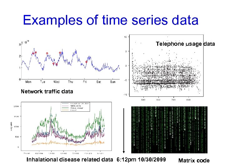Examples of time series data Telephone usage data Network traffic data Inhalational disease related data 6: 12 pm 10/30/2099 Matrix code

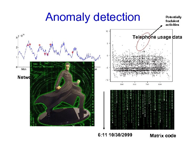Anomaly detection Potentially fradulent activities Telephone usage data Network traffic data 6: 11 10/30/2099 Matrix code

Applications • • Failure detection Fraud detection (credit card, telephone) Spam detection Biosurveillance – detecting geographic hotspots • Computer intrusion detection – detecting masqueraders

Time series • What is it about time series structure – Stationarity (e. g. , markov, exchangeability) – Typical stochastic process assumptions (e. g. , independent increment as in Poisson process) – Mixtures of above • Typical statistics involved – – Transition probabilities Event counts Mean, variance, spectral density, … Generally likelihood ratio of some kind Don’t worry if you don’t know all of these terminologies! • We shall try to exploit some of these structures in anomaly detection tasks

List of methods • • • clustering, dimensionality reduction mixture models Markov chain HMMs mixture of MC’s Poisson processes

Anomaly detection outline • Conceptual framework • Issues unique to anomaly detection – Feature engineering – Criteria in anomaly detection – Supervised vs unsupervised learning • Example: network anomaly detection using PCA • Intrusion detection – Detecting anomalies in multiple time series • Example: detecting masqueraders in multi-user systems

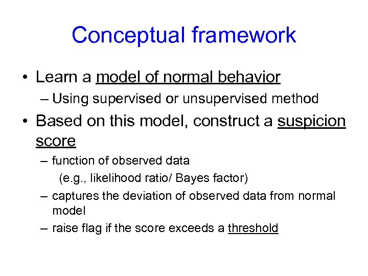Conceptual framework • Learn a model of normal behavior – Using supervised or unsupervised method • Based on this model, construct a suspicion score – function of observed data (e. g. , likelihood ratio/ Bayes factor) – captures the deviation of observed data from normal model – raise flag if the score exceeds a threshold

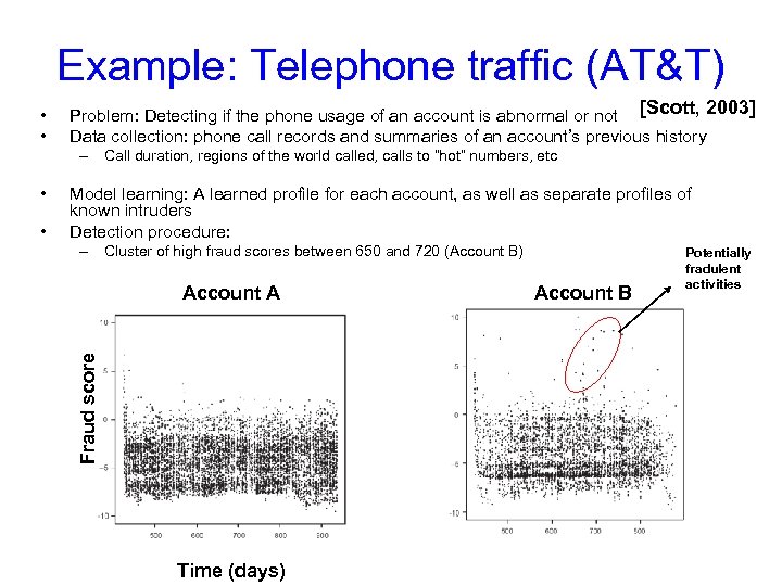Example: Telephone traffic (AT&T) • • Problem: Detecting if the phone usage of an account is abnormal or not [Scott, 2003] Data collection: phone call records and summaries of an account’s previous history – Call duration, regions of the world called, calls to “hot” numbers, etc • Model learning: A learned profile for each account, as well as separate profiles of known intruders Detection procedure: – Cluster of high fraud scores between 650 and 720 (Account B) Account A Fraud score • Time (days) Account B Potentially fradulent activities

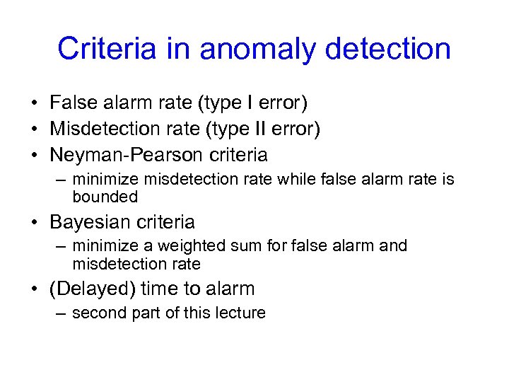Criteria in anomaly detection • False alarm rate (type I error) • Misdetection rate (type II error) • Neyman-Pearson criteria – minimize misdetection rate while false alarm rate is bounded • Bayesian criteria – minimize a weighted sum for false alarm and misdetection rate • (Delayed) time to alarm – second part of this lecture

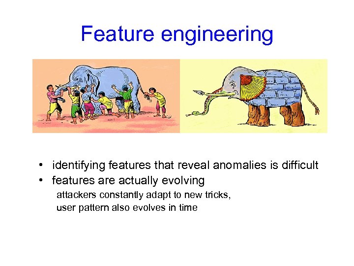Feature engineering • identifying features that reveal anomalies is difficult • features are actually evolving attackers constantly adapt to new tricks, user pattern also evolves in time

Feature choice by types of fraud • Example: Credit card/telephone fraud – stolen card: unusual spending within short amount of time – application fraud (using false information): first-time users, amount of spending – unusual called locations – “ghosting”: fraudster tricks the network to obtain free cards • Other domains: features might not be immediately indicative of normal/abnormal behavior

From features to models • More sophisticated test scores built upon aggregation of features – Dimensionality reduction methods • PCA, factor analysis, clustering – Methods based on probabilistic • Markov chain based, hidden markov models • etc

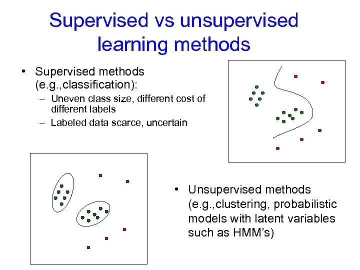Supervised vs unsupervised learning methods • Supervised methods (e. g. , classification): – Uneven class size, different cost of different labels – Labeled data scarce, uncertain • Unsupervised methods (e. g. , clustering, probabilistic models with latent variables such as HMM’s)

Example: Anomalies off the principal components[Lakhina et al, 2004] Abilene backbone network traffic volume over 41 links collected over 4 weeks Perform PCA on 41 -dim data Select top 5 components anomalies Network traffic data threshold Projection to residual subspace

Anomaly detection outline • Conceptual framework • Issues unique to anomaly detection • Example: network anomaly detection using PCA • Intrusion detection – Detecting anomalies in multiple time series • Example: detecting masqueraders in multi-user computer systems

Intrusion detection (multiple anomalies in multiple time series)

Broad spectrum of possibilities and difficulties • Trusted system users turning from legitimate usage to abuse of system resources • System penetration by sophisticated and careful hostile outsiders • One-time use by a co-worker “borrowing” a workstation • Automated penetrations by relatively naïve attacker via scripted attack sequences • Varying time spans from few seconds to months • Patterns might appear only in data gathered in distantly distributed sources • What sources? Command data, system call traces, network activity logs, CPU load averages, disk access patterns? • Data corrupted by noise or interspersed with examples of normal pattern usage

Intrusion detection • Each user has his own model (profile) – Known attacker profiles • Updating: Models describing user behavior allowed to evolve (slowly) – Reduce false alarm rate dramatically – Recent data more valuable than old ones

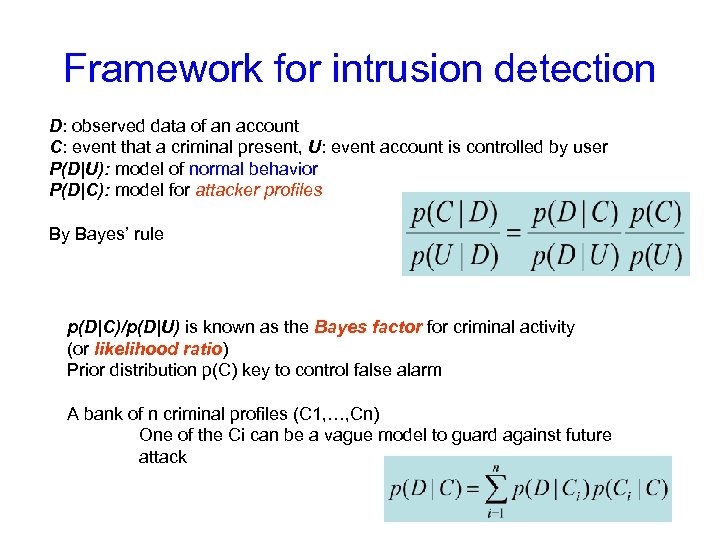Framework for intrusion detection D: observed data of an account C: event that a criminal present, U: event account is controlled by user P(D|U): model of normal behavior P(D|C): model for attacker profiles By Bayes’ rule p(D|C)/p(D|U) is known as the Bayes factor for criminal activity (or likelihood ratio) Prior distribution p(C) key to control false alarm A bank of n criminal profiles (C 1, …, Cn) One of the Ci can be a vague model to guard against future attack

Simple metrics • Some existing intrusion detection procedures not formally expressed as probabilistic models – one can often find stochastic models (under our framework) leading to the same detection procedures • Use of “distance metric” or statistic d(x) might correspond to – Gaussian p(x|U) = exp(-d(x)^2/2) – Laplace p(x|U) = exp(-d(x)) • Procedures based on event counts may often be represented as multinomial models

Intrusion detection outline • Conceptual framework of intrusion detection procedure • Example: Detecting masqueraders – Probabilistic models – how models are used for detection

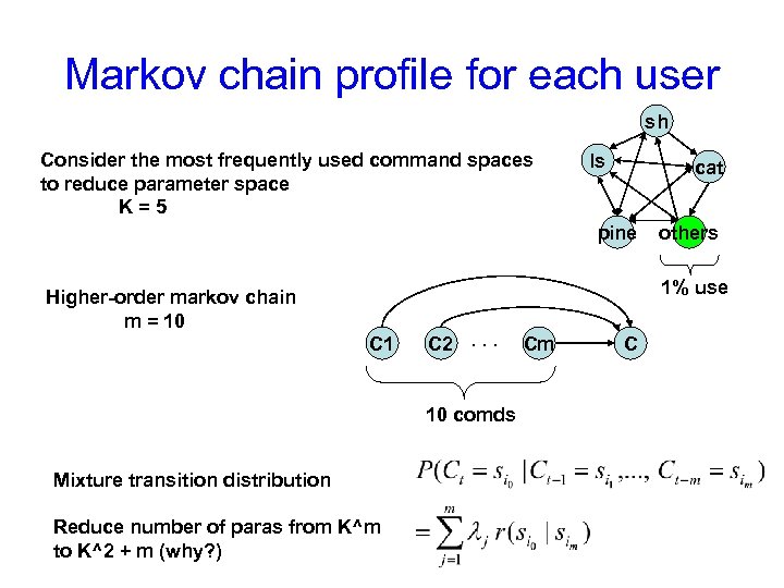
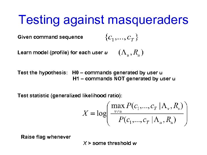
Markov chain based model for detecting masqueraders [Ju & Vardi, 99] • Modeling “signature behavior” for individual users based on system command sequences • High-order Markov structure is used – Takes into account last several commands instead of just the last one – Mixture transition distribution • Hypothesis test using generalized likelihood ratio

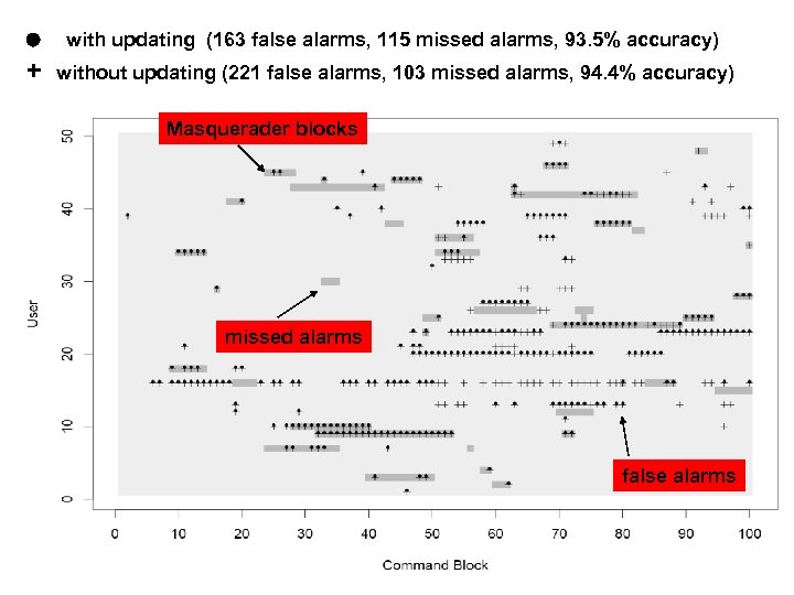
Data and experimental design • • Data consist of sequences of (unix) system commands and user names 70 users, 150, 000 consecutive commands each (=150 blocks of 100 commands) • • Randomly select 50 users to form a “community”, 20 outsiders First 50 blocks for training, next 100 blocks for testing • Starting after block 50, randomly insert command blocks from 20 outsiders – For each command block i (i=50, 51, . . . , 150), there is a prob 1% that some masquerading blocks inserted after it – The number x of command blocks inserted has geometric dist with mean 5 – Insert x blocks from an outside user, randomly chosen

Markov chain profile for each user sh Consider the most frequently used command spaces to reduce parameter space K=5 ls cat pine others 1% use Higher-order markov chain m = 10 C 1 C 2. . . 10 comds Mixture transition distribution Reduce number of paras from K^m to K^2 + m (why? ) Cm C

Testing against masqueraders Given command sequence Learn model (profile) for each user u Test the hypothesis: H 0 – commands generated by user u H 1 – commands NOT generated by user u Test statistic (generalized likelihood ratio): Raise flag whenever X > some threshold w

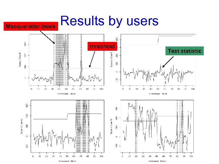
with updating (163 false alarms, 115 missed alarms, 93. 5% accuracy) + without updating (221 false alarms, 103 missed alarms, 94. 4% accuracy) Masquerader blocks missed alarms false alarms

Results by users Missed alarms threshold Masquerader block Test statistic False alarms

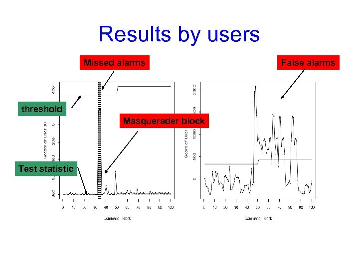
Masquerader block Results by users threshold Test statistic

Take-home message (again) • Learn a model of normal behavior for each monitored individuals • Based on this model, construct a suspicion score – function of observed data (e. g. , likelihood ratio/ Bayes factor) – captures the deviation of observed data from normal model – raise flag if the score exceeds a threshold

Other models in literature • Simple metrics – Hamming metric [Hofmeyr, Somayaji & Forest] – Sequence-match [Lane and Brodley] – IPAM (incremental probabilistic action modeling) [Davison and Hirsh] – PCA on transitional probability matrix [Du. Mouchel and Schonlau] • More elaborate probabilistic models – Bayes one-step Markov [Du. Mouchel] – Compression model – Mixture of Markov chains [Jha et al] • Elaborate probabilistic models can be used to obtain answer to more elaborate queries – Beyond yes/no question (see next slide)

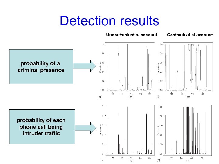
Burst modeling using Markov modulated Poisson process [Scott, 2003] Poisson process N 0 binary Markov chain Poisson process N 1 • • • can be also seen as a nonstationary discrete time HMM (thus all inferential machinary in HMM applies) requires less parameter (less memory) convenient to model sharing across time

Detection results Uncontaminated account probability of a criminal presence probability of each phone call being intruder traffic Contaminated account

Outline Anomaly detection with time series data Detecting bursts Sequential detection with time series data Detecting trends

Sequential analysis: balancing the tradeoff between detection accuracy and detection delay Xuan. Long Nguyen xuanlong@eecs. berkeley. edu Radlab, 11/06/06

Outline • Motivation in detection problems – need to minimize detection delay time • Brief intro to sequential analysis – sequential hypothesis testing – sequential change-point detection • Applications – Detection of anomalies in network traffic (network attacks), faulty software, etc

Three quantities of interest in detection problems • Detection accuracy – False alarm rate – Misdetection rate • Detection delay time

Network volume anomaly detection [Huang et al, 06]

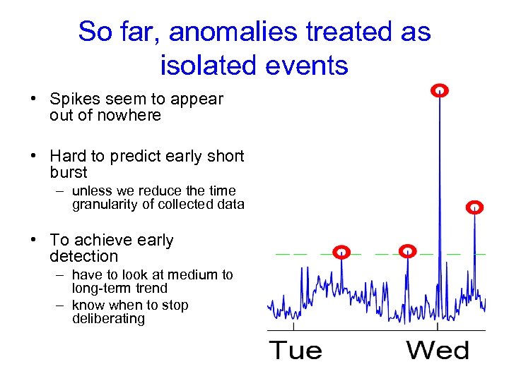So far, anomalies treated as isolated events • Spikes seem to appear out of nowhere • Hard to predict early short burst – unless we reduce the time granularity of collected data • To achieve early detection – have to look at medium to long-term trend – know when to stop deliberating

Early detection of anomalous trends • We want to – distinguish “bad” process from good process/ multiple processes – detect a point where a “good” process turns bad • Applicable when evidence accumulates over time (no matter how fast or slow) – e. g. , because a router or a server fails – worm propagates its effect • Sequential analysis is well-suited – minimize the detection time given fixed false alarm and misdetection rates – balance the tradeoff between these three quantities (false alarm, misdetection rate, detection time) effectively

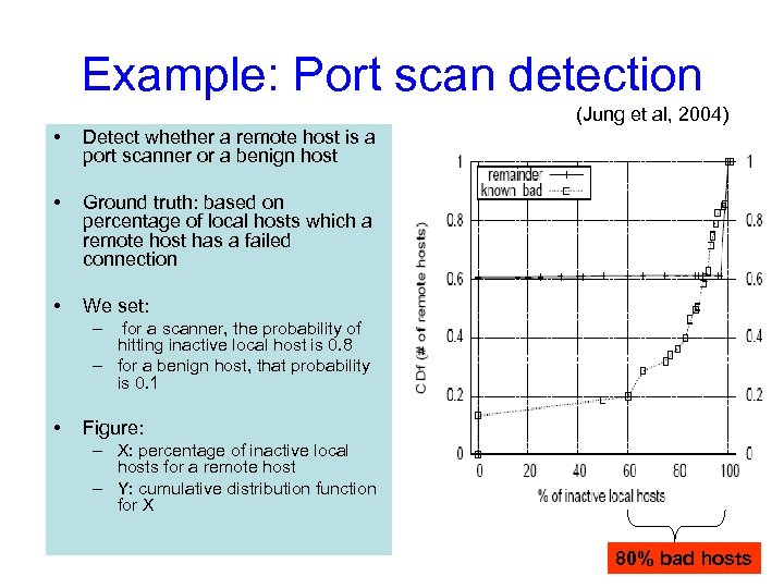Example: Port scan detection (Jung et al, 2004) • Detect whether a remote host is a port scanner or a benign host • Ground truth: based on percentage of local hosts which a remote host has a failed connection • We set: – for a scanner, the probability of hitting inactive local host is 0. 8 – for a benign host, that probability is 0. 1 • Figure: – X: percentage of inactive local hosts for a remote host – Y: cumulative distribution function for X 80% bad hosts

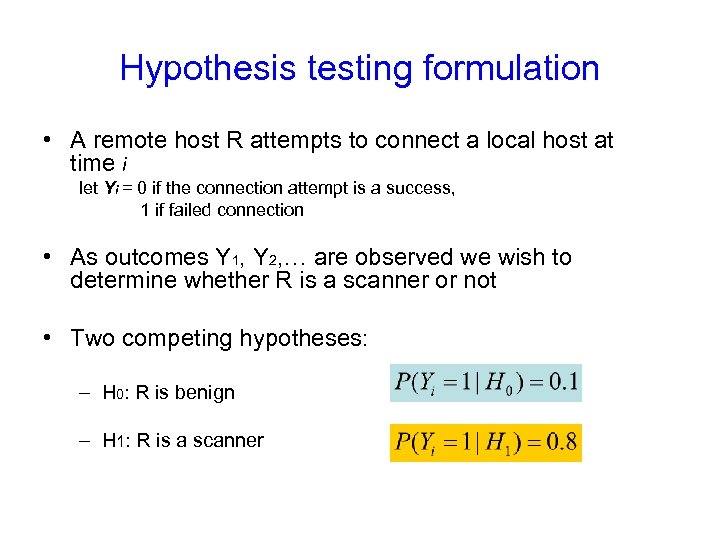Hypothesis testing formulation • A remote host R attempts to connect a local host at time i let Yi = 0 if the connection attempt is a success, 1 if failed connection • As outcomes Y 1, Y 2, … are observed we wish to determine whether R is a scanner or not • Two competing hypotheses: – H 0: R is benign – H 1: R is a scanner

An off-line approach 1. Collect sequence of data Y for one day (wait for a day) 2. Compute the likelihood ratio accumulated over a day This is related to the proportion of inactive local hosts that R tries to connect (resulting in failed connections) 3. Raise a flag if this statistic exceeds some threshold

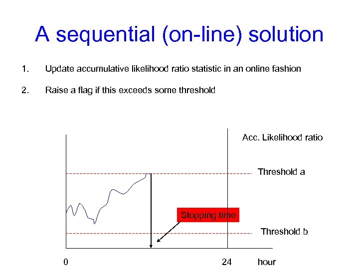A sequential (on-line) solution 1. Update accumulative likelihood ratio statistic in an online fashion 2. Raise a flag if this exceeds some threshold Acc. Likelihood ratio Threshold a Stopping time Threshold b 0 24 hour

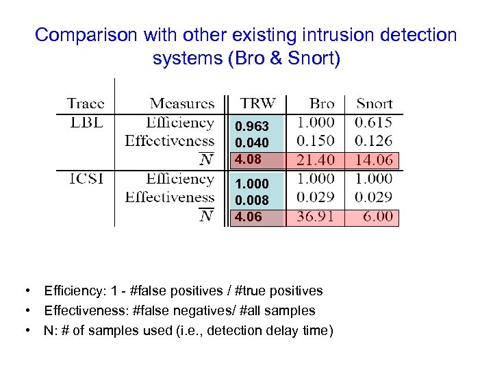Comparison with other existing intrusion detection systems (Bro & Snort) 0. 963 0. 040 4. 08 1. 000 0. 008 4. 06 • Efficiency: 1 - #false positives / #true positives • Effectiveness: #false negatives/ #all samples • N: # of samples used (i. e. , detection delay time)

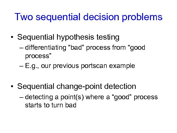Two sequential decision problems • Sequential hypothesis testing – differentiating “bad” process from “good process” – E. g. , our previous portscan example • Sequential change-point detection – detecting a point(s) where a “good” process starts to turn bad

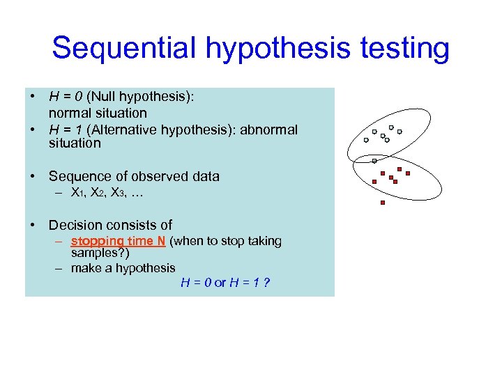Sequential hypothesis testing • H = 0 (Null hypothesis): normal situation • H = 1 (Alternative hypothesis): abnormal situation • Sequence of observed data – X 1, X 2, X 3, … • Decision consists of – stopping time N (when to stop taking samples? ) – make a hypothesis H = 0 or H = 1 ?

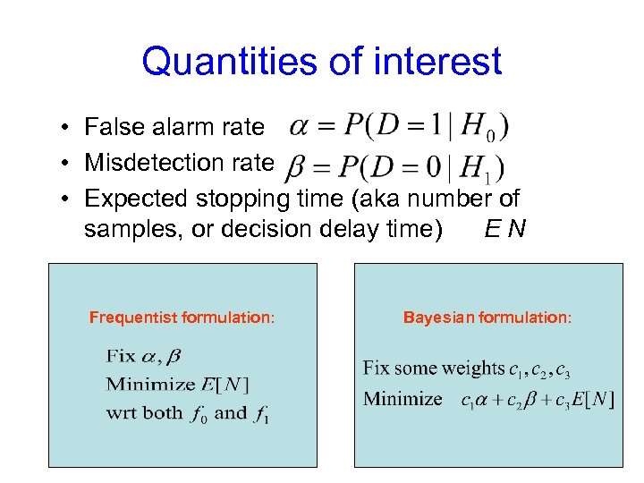Quantities of interest • False alarm rate • Misdetection rate • Expected stopping time (aka number of samples, or decision delay time) EN Frequentist formulation: Bayesian formulation:

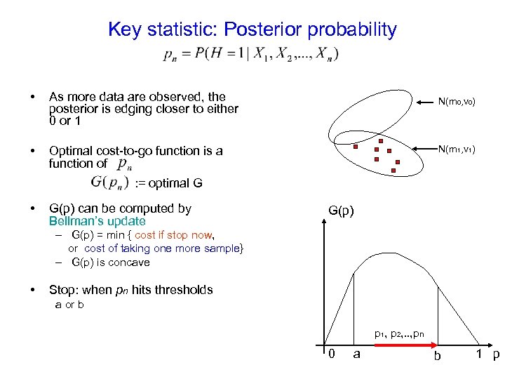Key statistic: Posterior probability • As more data are observed, the posterior is edging closer to either 0 or 1 • Optimal cost-to-go function is a function of N(m 0, v 0) N(m 1, v 1) : = optimal G • G(p) can be computed by Bellman’s update G(p) – G(p) = min { cost if stop now, or cost of taking one more sample} – G(p) is concave • Stop: when pn hits thresholds a or b p 1, p 2, . . , pn 0 a b 1 p

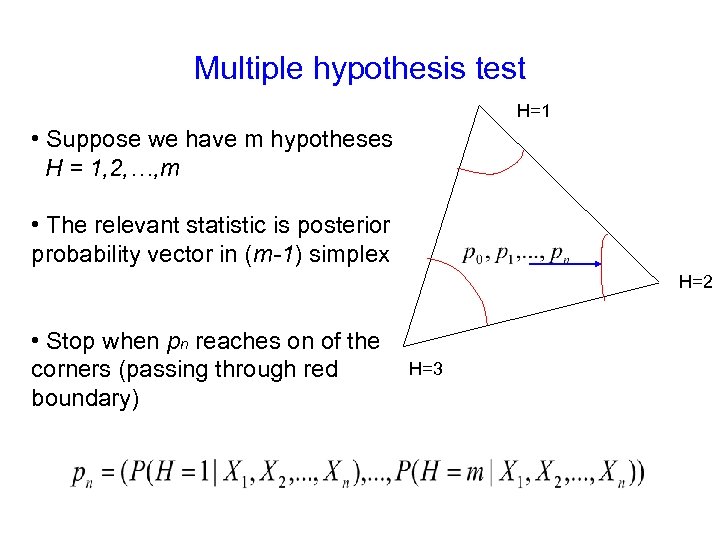Multiple hypothesis test H=1 • Suppose we have m hypotheses H = 1, 2, …, m • The relevant statistic is posterior probability vector in (m-1) simplex H=2 • Stop when pn reaches on of the corners (passing through red boundary) H=3

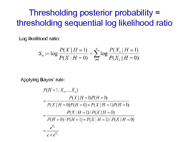Thresholding posterior probability = thresholding sequential log likelihood ratio Log likelihood ratio: Applying Bayes’ rule:

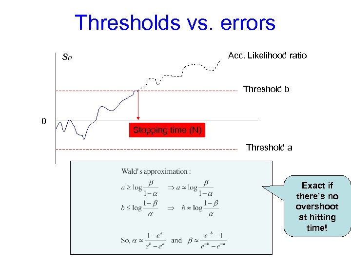Thresholds vs. errors Acc. Likelihood ratio Sn Threshold b 0 Stopping time (N) Threshold a Exact if there’s no overshoot at hitting time!

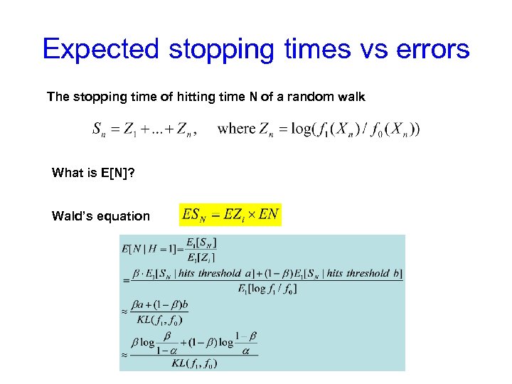Expected stopping times vs errors The stopping time of hitting time N of a random walk What is E[N]? Wald’s equation

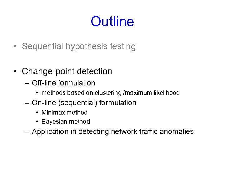Outline • Sequential hypothesis testing • Change-point detection – Off-line formulation • methods based on clustering /maximum likelihood – On-line (sequential) formulation • Minimax method • Bayesian method – Application in detecting network traffic anomalies

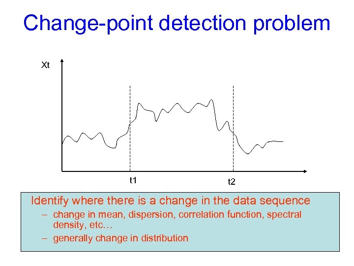Change-point detection problem Xt t 1 t 2 Identify where there is a change in the data sequence – change in mean, dispersion, correlation function, spectral density, etc… – generally change in distribution

Off-line change-point detection • Viewed as a clustering problem across time axis – Change points being the boundary of clusters • Partition time series data that respects – Homogeneity within a partition – Heterogeneity between partitions

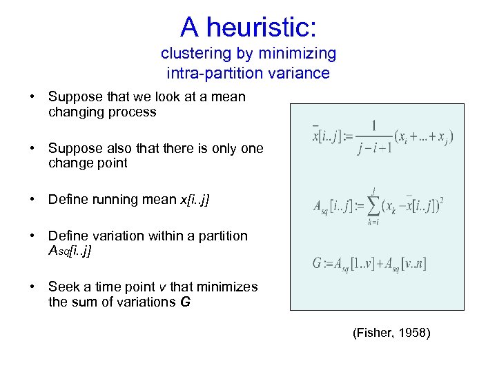A heuristic: clustering by minimizing intra-partition variance • Suppose that we look at a mean changing process • Suppose also that there is only one change point • Define running mean x[i. . j] • Define variation within a partition Asq[i. . j] • Seek a time point v that minimizes the sum of variations G (Fisher, 1958)

Statistical inference of change point • A change point is considered as a latent variable • Statistical inference of change point location via – frequentist method, e. g. , maximum likelihood estimation – Bayesian method by inferring posterior probability

Maximum-likelihood method [Page, 1965] Hypothesis Hv: sequence has density f 0 before v, and f 1 after This is the precursor for various sequential procedures (to come!) Hypothesis H 0: sequence is stochastically homogeneous Sk 1 f 0 v n k

Maximum-likelihood method [Hinkley, 1970, 1971]

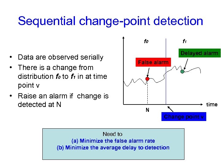Sequential change-point detection f 0 • Data are observed serially • There is a change from distribution f 0 to f 1 in at time point v • Raise an alarm if change is detected at N f 1 Delayed alarm False alarm time N Change point v Need to (a) Minimize the false alarm rate (b) Minimize the average delay to detection

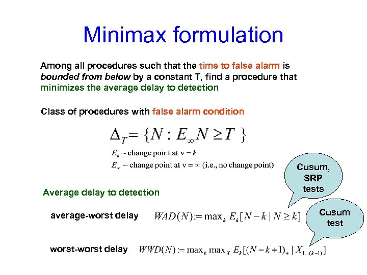Minimax formulation Among all procedures such that the time to false alarm is bounded from below by a constant T, find a procedure that minimizes the average delay to detection Class of procedures with false alarm condition Average delay to detection average-worst delay worst-worst delay Cusum, SRP tests Cusum test

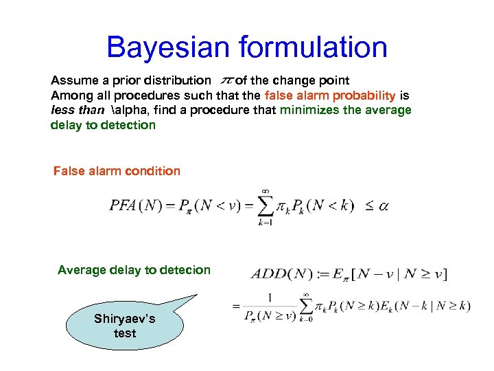Bayesian formulation Assume a prior distribution of the change point Among all procedures such that the false alarm probability is less than alpha, find a procedure that minimizes the average delay to detection False alarm condition Average delay to detecion Shiryaev’s test

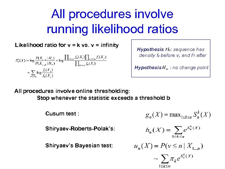All procedures involve running likelihood ratios Likelihood ratio for v = k vs. v = infinity Hypothesis Hv: sequence has density f 0 before v, and f 1 after Hypothesis : no change point All procedures involve online thresholding: Stop whenever the statistic exceeds a threshold b Cusum test : Shiryaev-Roberts-Polak’s: Shiryaev’s Bayesian test:

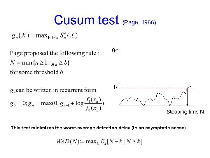Cusum test (Page, 1966) gn b Stopping time N This test minimizes the worst-average detection delay (in an asymptotic sense) :

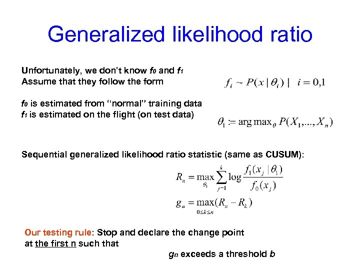Generalized likelihood ratio Unfortunately, we don’t know f 0 and f 1 Assume that they follow the form f 0 is estimated from “normal” training data f 1 is estimated on the flight (on test data) Sequential generalized likelihood ratio statistic (same as CUSUM): Our testing rule: Stop and declare the change point at the first n such that gn exceeds a threshold b

Change point detection in network traffic N(m 0, v 0) [Hajji, 2005] N(m 1, v 1) N(m, v) Data features: Changed behavior number of good packets received that were directed to the broadcast address number of Ethernet packets with an unknown protocol type number of good address resolution protocol (ARP) packets on the segment number of incoming TCP connection requests (TCP packets with SYN flag set) Each feature is modeled as a mixture of 3 -4 gaussians to adjust to the daily traffic patterns (night hours vs day times, weekday vs. weekends, …)

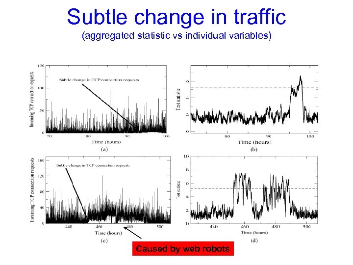Subtle change in traffic (aggregated statistic vs individual variables) Caused by web robots

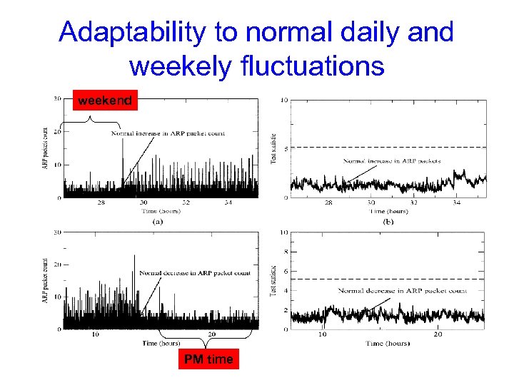Adaptability to normal daily and weekely fluctuations weekend PM time

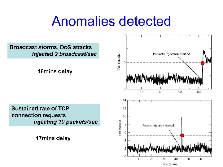Anomalies detected Broadcast storms, Do. S attacks injected 2 broadcast/sec 16 mins delay Sustained rate of TCP connection requests injecting 10 packets/sec 17 mins delay

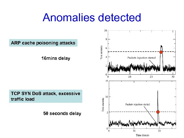Anomalies detected ARP cache poisoning attacks 16 mins delay TCP SYN Do. S attack, excessive traffic load 50 seconds delay

Summary • Sequential hypothesis test – distinguish “good” process from “bad” • Sequential change-point detection – detecting where a process changes its behavior • Framework for optimal reduction of detection delay • Sequential tests are very easy to apply – even though the analysis might look difficult

References for anomaly detection • • Schonlau, M, Du. Mouchel W, Ju W, Karr, A, theus, M and Vardi, Y. Computer instrusion: Detecting masquerades, Statistical Science, 2001. Jha S, Kruger L, Kurtz, T, Lee, Y and Smith A. A filtering approach to anomaly and masquerade detection. Technical report, Univ of Wisconsin, Madison. Scott, S. , A Bayesian paradigm for designing intrusion detection systems. Computational Statistics and Data Analysis, 2003. Bolton R. and Hand, D. Statistical fraud detection: A review. Statistical Science, Vol 17, No 3, 2002, Ju, W and Vardi Y. A hybrid high-order Markov chain model for computer intrusion detection. Tech Report 92, National Institute Statistical Sciences, 1999. Lane, T and Brodley, C. E. Approaches to online learning and concept drift for user identification in computer security. Proc. KDD, 1998. Lakhina A, Crovella, M and Diot, C. diagnosing network-wide traffic anomalies. ACM Sigcomm, 2004

References for sequential analysis • • • Wald, A. Sequential analysis, John Wiley and Sons, Inc, 1947. Arrow, K. , Blackwell, D. , Girshik, Ann. Math. Stat. , 1949. Shiryaev, R. Optimal stopping rules, Springer-Verlag, 1978. Siegmund, D. Sequential analysis, Springer-Verlag, 1985. Brodsky, B. E. and Darkhovsky B. S. Nonparametric methods in change-point problems. Kluwer Academic Pub, 1993. Baum, C. W. & Veeravalli, V. V. A Sequential Procedure for Multihypothesis Testing. IEEE Trans on Info Thy, 40(6)1994 -2007, 1994. Lai, T. L. , Sequential analysis: Some classical problems and new challenges (with discussion), Statistica Sinica, 11: 303— 408, 2001. Mei, Y. Asymptotically optimal methods for sequential change-point detection, Caltech Ph. D thesis, 2003. Hajji, H. Statistical analysis of network traffic for adaptive faults detection, IEEE Trans Neural Networks, 2005. Tartakovsky, A & Veeravalli, V. V. General asymptotic Bayesian theory of quickest change detection. Theory of Probability and Its Applications, 2005 Nguyen, X. , Wainwright, M. & Jordan, M. I. On optimal quantization rules in sequential decision problems. Proc. ISIT, Seattle, 2006.