

d7dbedb97e85b036dc65b41fb1bb059f.ppt
- Количество слайдов: 92
 Analyzing Your Data with Analytic Functions Carl Dudley University of Wolverhampton, UK UKOUG Council Oracle ACE Director carl. dudley@wlv. ac. uk
 Introduction Working with Oracle since 1986 Oracle DBA - OCP Oracle 7, 8, 9, 10 Oracle DBA of the Year – 2002 Oracle ACE Director Regular Presenter at Oracle Conferences Consultant and Trainer Technical Editor for a number of Oracle texts UK Oracle User Group Council Member of IOUC Day job – University of Wolverhampton, UK Carl Dudley University of Wolverhampton, UK 2
 Analyzing Your Data with Analytic Functions Overview of Analytic Functions Ranking Functions Partitioning Aggregate Functions Sliding Windows Row Comparison Functions Analytic Function Performance Carl Dudley University of Wolverhampton, UK 3
 Analytic Functions Ø New set of functions introduced in Oracle 8. 1. 6 — Analytic functions or Window functions Ø Intended for OLAP (On. Line Analytic Processing) or data warehouse purposes Ø Provide functionality that would require complex conventional SQL programming or other tools Ø Advantages — Improved performance • The optimizer “understands” the purpose of the query — Reduced dependency on report generators and client tools — Simpler coding Carl Dudley University of Wolverhampton, UK 4
 Analytic Function Categories Ø The analytic functions fall into four categories Ranking functions Aggregate functions Row comparison functions Statistical functions Ø The Oracle documentation describes all of the functions Ø Processed as the last step before ORDER BY — Work on the result set of the query — Can operate on an intermediate ordering of the rows — Actions can be based on : • Partitions of the result set • A sliding window of rows in the result set Carl Dudley University of Wolverhampton, UK 5
 Processing Sequence Ø There may be several intermediate sort steps if required Analytic process Rows WHERE evaluation GROUPING HAVING evaluation Intermediate ordering Analytic function Final ORDER BY Carl Dudley University of Wolverhampton, UK Output 6
 OVER(<analytic clause>) Ø The enclosing parentheses are") The Analytic Clause Ø Syntax :
The Analytic Clause Ø Syntax :
 Sequence of Processing Ø Being processed just before the final ORDER BY means : — Analytic functions are not allowed in WHERE and HAVING conditions • Allowed only in the final ORDER BY clause Ø Ordering the final result set — OVER clause specifies sort order of result set before analytic function is computed — Can have multiple analytic functions with different OVER clauses, requiring multiple intermediate sorts — Final ordering does not have to match ordering in OVER clause Carl Dudley University of Wolverhampton, UK 8
 The emp and dept Tables Analytic Functions emp DEPTNO DNAME LOC ---------- 10 ACCOUNTING NEW YORK 20 RESEARCH DALLAS 30 SALES CHICAGO Overview of Analytic Functions 40 OPERATIONS BOSTON dept EMPNO ENAME JOB MGR HIREDATE SAL COMM DEPTNO --------- ----- -----Partitioning 7934 MILLER CLERK 7782 23 -JAN-1982 1300 10 7782 CLARK MANAGER 7839 09 -JUN-1981 2450 10 7839 KING PRESIDENT 17 -NOV-1981 5000 10 Aggregate Functions 7369 SMITH CLERK 7902 17 -DEC-1980 800 20 7876 ADAMS CLERK 7788 12 -JAN-1983 1100 20 Sliding Windows 7566 JONES MANAGER 7839 02 -APR-1981 2975 20 7902 FORD ANALYST 7566 03 -DEC-1981 3000 20 7788 SCOTT ANALYST 7566 09 -DEC-1982 3000 20 Row Comparison Functions 7900 JAMES CLERK 7698 03 -DEC-1981 950 30 7521 WARD SALESMAN 7698 22 -FEB-1981 1250 500 30 7654 MARTIN SALESMAN 7698 28 -SEP-1981 1250 1400 30 Analytic Function Performance 7844 TURNER SALESMAN 7698 08 -SEP-1981 1500 0 30 7499 ALLEN SALESMAN 7698 20 -FEB-1981 1600 300 30 7698 BLAKE MANAGER 7839 01 -MAY-1981 2850 30 Ranking Functions Carl Dudley University of Wolverhampton, UK 9
 Example of Ranking Ø Ranking with ROW_NUMBER — No handling of ties • Rows retrieved by the query are intermediately sorted on descending salary for the analysis SELECT ROW_NUMBER() OVER( ORDER BY sal DESC) rownumber , sal , ename FROM emp ORDER BY sal DESC; — If the final ORDER BY specifies the same sort order as the OVER clause only one sort is required — ROW_NUMBER is different from ROWNUMBER SAL ENAME ----- 1 5000 KING 2 3000 SCOTT 3 3000 FORD 4 2975 JONES 5 2850 BLAKE 6 2450 CLARK 7 1600 ALLEN 8 1500 TURNER 9 1300 MILLER 10 1250 WARD 11 1250 MARTIN 12 1100 ADAMS 13 950 JAMES 14 800 SMITH Carl Dudley University of Wolverhampton, UK 10
 Different Sort Order in Final ORDER BY Ø If the OVER clause sort is different from the final ORDER BY — An extra sort step is required SELECT ROW_NUMBER() OVER( ORDER BY sal DESC) rownumber , sal , ename FROM emp ORDER BY ename; ROWNUMBER SAL ENAME ----- 12 1100 ADAMS 7 1600 ALLEN 5 2850 BLAKE 6 2450 CLARK 3 3000 FORD 13 950 JAMES 4 2975 JONES 1 5000 KING 11 1250 MARTIN 9 1300 MILLER 2 3000 SCOTT 14 800 SMITH 8 1500 TURNER 10 1250 WARD Carl Dudley University of Wolverhampton, UK 11
 Multiple Functions With Different Sort Order Ø Multiple OVER clauses can be used SELECT ROW_NUMBER() OVER(ORDER BY sal DESC) sal_n , sal , ROW_NUMBER() OVER(ORDER BY comm DESC NULLS LAST) comm_n , comm , ename FROM emp ORDER BY ename; Carl Dudley University of Wolverhampton, UK 12
 RANK and DENSE_RANK Ø ROW_NUMBER increases even if several rows have identical values — Does not handle ties Ø RANK and DENSE_RANK handle ties — Rows with the same value are given the same rank — After the tie value, RANK skips numbers, DENSE_RANK does not Ø Ranking using analytic functions has better performance, because the table is not read repeatedly Carl Dudley University of Wolverhampton, UK 13
 SELECT ROW_NUMBER() OVER(ORDER BY sal DESC) rownumber , RANK() OVER(ORDER") RANK and DENSE_RANK (continued) SELECT ROW_NUMBER() OVER(ORDER BY sal DESC) rownumber , RANK() OVER(ORDER BY sal DESC) rank , DENSE_RANK() OVER(ORDER BY sal DESC) denserank , sal , ename FROM emp ORDER BY sal DESC, ename; ROWNUMBER RANK DENSERANK SAL ENAME ---------- 1 1 5000 KING 2 2 3000 FORD 3 2 2 3000 SCOTT 4 4 3 2975 JONES 5 5 4 2850 BLAKE 6 6 5 2450 CLARK 7 7 6 1600 ALLEN 8 8 7 1500 TURNER 9 9 8 1300 MILLER 10 9 1250 MARTIN 11 10 9 1250 WARD 12 10 1100 ADAMS 13 11 950 JAMES 14 12 800 SMITH Multiple OVER clauses may be used specifying different orderings Carl Dudley University of Wolverhampton, UK 14
RANK and DENSE_RANK (continued) SELECT ROW_NUMBER() OVER(ORDER BY sal DESC) rownumber , RANK() OVER(ORDER BY sal DESC) rank , DENSE_RANK() OVER(ORDER BY sal DESC) denserank , sal , ename FROM emp ORDER BY sal DESC, ename; ROWNUMBER RANK DENSERANK SAL ENAME ---------- 1 1 5000 KING 2 2 3000 FORD 3 2 2 3000 SCOTT 4 4 3 2975 JONES 5 5 4 2850 BLAKE 6 6 5 2450 CLARK 7 7 6 1600 ALLEN 8 8 7 1500 TURNER 9 9 8 1300 MILLER 10 9 1250 MARTIN 11 10 9 1250 WARD 12 10 1100 ADAMS 13 11 950 JAMES 14 12 800 SMITH Multiple OVER clauses may be used specifying different orderings Carl Dudley University of Wolverhampton, UK 14
 Analytic Function in ORDER BY Ø Analytic functions are computed before the final ordering — Can be referenced in the final ORDER BY clause — An alias is used in this case SELECT RANK() OVER( ORDER BY sal DESC) sal_rank , sal , ename FROM emp ORDER BY sal_rank , ename; SAL_RANK SAL ENAME ----- 1 5000 KING 2 3000 FORD 2 3000 SCOTT 4 2975 JONES 5 2850 BLAKE 6 2450 CLARK 7 1600 ALLEN 8 1500 TURNER 9 1300 MILLER 10 1250 MARTIN 10 1250 WARD 12 1100 ADAMS 13 950 JAMES 14 800 SMITH Carl Dudley University of Wolverhampton, UK 15
 functions are computed after the WHERE condition and hence") WHERE Conditions Ø Analytic (window) functions are computed after the WHERE condition and hence not available in the WHERE clause SELECT RANK() OVER(ORDER BY sal DESC) rank , sal , ename FROM emp WHERE RANK() OVER(ORDER BY sal DESC) <= 5 ORDER BY rank WHERE RANK() OVER(ORDER BY sal DESC) <= 5 * ERROR at line 5: ORA-30483: window functions are not allowed here Carl Dudley University of Wolverhampton, UK 16
WHERE Conditions Ø Analytic (window) functions are computed after the WHERE condition and hence not available in the WHERE clause SELECT RANK() OVER(ORDER BY sal DESC) rank , sal , ename FROM emp WHERE RANK() OVER(ORDER BY sal DESC) <= 5 ORDER BY rank WHERE RANK() OVER(ORDER BY sal DESC) <= 5 * ERROR at line 5: ORA-30483: window functions are not allowed here Carl Dudley University of Wolverhampton, UK 16
 Ø Use an inline view to force the early processing of") WHERE Conditions (continued) Ø Use an inline view to force the early processing of the analytic SELECT * FROM (SELECT RANK() OVER(ORDER BY sal DESC) rank , sal , ename FROM emp) WHERE rank <= 5 ORDER BY rank , ename; RANK SAL ENAME ---------- 1 5000 KING 2 3000 FORD 2 3000 SCOTT 4 2975 JONES 5 2850 BLAKE — Inline view is processed before the WHERE clause Carl Dudley University of Wolverhampton, UK 17
WHERE Conditions (continued) Ø Use an inline view to force the early processing of the analytic SELECT * FROM (SELECT RANK() OVER(ORDER BY sal DESC) rank , sal , ename FROM emp) WHERE rank <= 5 ORDER BY rank , ename; RANK SAL ENAME ---------- 1 5000 KING 2 3000 FORD 2 3000 SCOTT 4 2975 JONES 5 2850 BLAKE — Inline view is processed before the WHERE clause Carl Dudley University of Wolverhampton, UK 17
 Grouping, Aggregate Functions and Analytics Ø Rank the departments by number of employees SELECT deptno , COUNT(*) employees , RANK() OVER(ORDER BY COUNT(*) DESC) rank FROM emp GROUP BY deptno ORDER BY employees , deptno; DEPTNO EMPLOYEES RANK ---------- 10 3 20 5 2 30 6 1 Ø Analytic functions are illegal in the HAVING clause — The workaround is the same; use an inline view — Ordering subclause may not reference a column alias Carl Dudley University of Wolverhampton, UK 18
 Analytic Functions Overview of Analytic Functions Ranking Functions Partitioning Aggregate Functions Sliding Windows Row Comparison Functions Analytic Function Performance Carl Dudley University of Wolverhampton, UK 19
 Partitioning Ø Analytic functions can be applied to logical groups within the result set rather than the full result set — Partitions. . . OVER(PARTITION BY mgr ORDER BY sal DESC) — PARTITION BY specifies the grouping — ORDER BY specifies the ordering within each group — Not connected with database table partitioning Ø If partitioning is not specified, the full result set behaves as one partition Ø NULL values are grouped together in one partition, as in GROUP BY Ø Can have multiple analytic functions with different partitioning subclauses Carl Dudley University of Wolverhampton, UK 20
 Partitioning Example Ø Rank employees by salary within their manager SELECT ename , mgr , sal , RANK() OVER(PARTITION BY mgr ORDER BY sal DESC) m_rank FROM emp ORDER BY mgr , m_rank; ENAME MGR SAL M_RANK ---------- -----SCOTT 7566 3000 1 FORD 7566 3000 1 ALLEN 7698 1600 1 TURNER 7698 1500 2 WARD 7698 1250 3 MARTIN 7698 1250 3 JAMES 7698 950 5 MILLER 7782 1300 1 ADAMS 7788 1100 1 JONES 7839 2975 1 BLAKE 7839 2850 2 CLARK 7839 2450 3 SMITH 7902 800 1 KING 5000 1 Carl Dudley University of Wolverhampton, UK 21
 Result Sets With Different Partitioning Ø Rank the employees by salary within their manager, within the year they were hired, as well as overall SELECT ename , sal , manager , RANK() OVER(PARTITION BY mgr ORDER BY sal DESC) m_rank , TRUNC(TO_NUMBER(TO_CHAR(date_hired, 'YYYY'))) year_hired , RANK() OVER(PARTITION BY TRUNC(TO_NUMBER(TO_CHAR(date_hired, 'YYYY')) ORDER BY sal DESC) d_rank , RANK() OVER(ORDER BY sal DESC) rank FROM emp ORDER BY rank , ename; Carl Dudley University of Wolverhampton, UK 22
 ENAME SAL MGR M_RANK YEAR_HIRED D_RANK ------- ----------KING") Result Sets With Different Partitioning (continued) ENAME SAL MGR M_RANK YEAR_HIRED D_RANK ------- ----------KING 5000 1 1981 1 FORD 3000 7566 1 1981 2 SCOTT 3000 7566 1 1987 1 2 JONES 2975 7839 1 1981 3 4 BLAKE 2850 7839 2 1981 4 5 CLARK 2450 7839 3 1981 5 6 ALLEN 1600 7698 1 1981 6 7 TURNER 1500 7698 2 1981 7 8 MILLER 1300 7782 1 1982 1 9 MARTIN 1250 7698 3 1981 8 10 WARD 1250 7698 3 1981 8 10 ADAMS 1100 7788 1 1987 2 12 JAMES 950 7698 5 1981 10 13 SMITH 800 7902 1 1980 14 Carl Dudley University of Wolverhampton, UK 23
Result Sets With Different Partitioning (continued) ENAME SAL MGR M_RANK YEAR_HIRED D_RANK ------- ----------KING 5000 1 1981 1 FORD 3000 7566 1 1981 2 SCOTT 3000 7566 1 1987 1 2 JONES 2975 7839 1 1981 3 4 BLAKE 2850 7839 2 1981 4 5 CLARK 2450 7839 3 1981 5 6 ALLEN 1600 7698 1 1981 6 7 TURNER 1500 7698 2 1981 7 8 MILLER 1300 7782 1 1982 1 9 MARTIN 1250 7698 3 1981 8 10 WARD 1250 7698 3 1981 8 10 ADAMS 1100 7788 1 1987 2 12 JAMES 950 7698 5 1981 10 13 SMITH 800 7902 1 1980 14 Carl Dudley University of Wolverhampton, UK 23
 in a group ('what-if' query)") Hypothetical Rank Ø Rank a specified hypothetical value (2999) in a group ('what-if' query) SELECT RANK(2999) WITHIN GROUP (ORDER BY sal DESC) H_S_rank , PERCENT_RANK(2999) WITHIN GROUP (ORDER BY sal DESC) PR , CUME_DIST(2999) WITHIN GROUP (ORDER BY sal DESC) CD FROM emp; H_S_RANK PR CD ---------- 4. 214285714. 266666667 3/14 4/15 SELECT deptno , RANK(20, 'CLERK') WITHIN GROUP (ORDER BY deptno DESC, job ASC) H_D_J_rank FROM emp GROUP BY deptno; A clerk in 20 would be higher than anyone in 10 DEPTNO H_D_J_RANK A clerk would be third in ascending job ---------order in department 20 (below analysts) 10 1 20 3 A clerk in 20 would be lower than anyone in 30 (6 employees) 30 7 Carl Dudley University of Wolverhampton, UK 24
Hypothetical Rank Ø Rank a specified hypothetical value (2999) in a group ('what-if' query) SELECT RANK(2999) WITHIN GROUP (ORDER BY sal DESC) H_S_rank , PERCENT_RANK(2999) WITHIN GROUP (ORDER BY sal DESC) PR , CUME_DIST(2999) WITHIN GROUP (ORDER BY sal DESC) CD FROM emp; H_S_RANK PR CD ---------- 4. 214285714. 266666667 3/14 4/15 SELECT deptno , RANK(20, 'CLERK') WITHIN GROUP (ORDER BY deptno DESC, job ASC) H_D_J_rank FROM emp GROUP BY deptno; A clerk in 20 would be higher than anyone in 10 DEPTNO H_D_J_RANK A clerk would be third in ascending job ---------order in department 20 (below analysts) 10 1 20 3 A clerk in 20 would be lower than anyone in 30 (6 employees) 30 7 Carl Dudley University of Wolverhampton, UK 24
 Ø Typical question — When a customer buys product x, how") Frequent Itemsets (dbms_frequent_itemset) Ø Typical question — When a customer buys product x, how likely are they to also buy product y? SELECT CAST(itemset AS fi_char) itemset , support , length , total_tranx FROM TABLE(DBMS_FREQUENT_ITEMSET. FI_TRANSACTIONAL( CURSOR(SELECT TO_CHAR(sales. cust_id) , TO_CHAR(sales. prod_id) Minimum fraction of different FROM sh. sales 'Documentation' customers , sh. products having this combination WHERE products. prod_id = sales. prod_id AND products. prod_subcategory = 'Documentation'), 0. 5, mimimum items in set 2, include items 3, Number of maximum items in set NULL, Different customers exclude items NULL)); ITEMSET SUPPORT LENGTH TOTAL_TRANX ------------------- -----FI_CHAR('40', '41') 3692 2 6077 2 or 3 items per set FI_CHAR('40', '42') 3900 2 6077 FI_CHAR('40', '45') 3482 2 6077 FI_CHAR('41', '42') 3163 2 6077 Number of instances FI_CHAR('40', '41', '42') 3141 3 6077 Carl Dudley University of Wolverhampton, UK 25
Frequent Itemsets (dbms_frequent_itemset) Ø Typical question — When a customer buys product x, how likely are they to also buy product y? SELECT CAST(itemset AS fi_char) itemset , support , length , total_tranx FROM TABLE(DBMS_FREQUENT_ITEMSET. FI_TRANSACTIONAL( CURSOR(SELECT TO_CHAR(sales. cust_id) , TO_CHAR(sales. prod_id) Minimum fraction of different FROM sh. sales 'Documentation' customers , sh. products having this combination WHERE products. prod_id = sales. prod_id AND products. prod_subcategory = 'Documentation'), 0. 5, mimimum items in set 2, include items 3, Number of maximum items in set NULL, Different customers exclude items NULL)); ITEMSET SUPPORT LENGTH TOTAL_TRANX ------------------- -----FI_CHAR('40', '41') 3692 2 6077 2 or 3 items per set FI_CHAR('40', '42') 3900 2 6077 FI_CHAR('40', '45') 3482 2 6077 FI_CHAR('41', '42') 3163 2 6077 Number of instances FI_CHAR('40', '41', '42') 3141 3 6077 Carl Dudley University of Wolverhampton, UK 25
 Ø Need to create type to accommodate the set — Ranking") Frequent Itemsets (continued) Ø Need to create type to accommodate the set — Ranking functions can be applied to the itemset CREATE TYPE fi_char AS TABLE OF VARCHAR 2(100); Ø The total transactions (TOTAL_TRANX) is the number of different customers involved with any product within the set of products under examination SELECT COUNT(DISTINCT cust_id) FROM sales prod_ids for WHERE prod_id BETWEEN 40 AND 45; 'Documentation' COUNT(DISTINCTCUST_ID) ----------- 6077 — Ranking functions can be applied to the itemset Ø Itemsets containing certain items can be included/excluded , CURSOR(SELECT * FROM table(fi_char(40, 45))) , CURSOR(SELECT * FROM table(fi_char(42))) Include any sets involving 40 or 45 Exclude any sets involving 42 Carl Dudley University of Wolverhampton, UK 26
Frequent Itemsets (continued) Ø Need to create type to accommodate the set — Ranking functions can be applied to the itemset CREATE TYPE fi_char AS TABLE OF VARCHAR 2(100); Ø The total transactions (TOTAL_TRANX) is the number of different customers involved with any product within the set of products under examination SELECT COUNT(DISTINCT cust_id) FROM sales prod_ids for WHERE prod_id BETWEEN 40 AND 45; 'Documentation' COUNT(DISTINCTCUST_ID) ----------- 6077 — Ranking functions can be applied to the itemset Ø Itemsets containing certain items can be included/excluded , CURSOR(SELECT * FROM table(fi_char(40, 45))) , CURSOR(SELECT * FROM table(fi_char(42))) Include any sets involving 40 or 45 Exclude any sets involving 42 Carl Dudley University of Wolverhampton, UK 26
 Plan of Itemset Query Ø Only one full table scan of sales ----------------------------------------|Id | Operation | Name |Rows | ----------------------------------------| 0| SELECT STATEMENT | 8| | 1| FIC RECURSIVE ITERATION | | | 2| FIC LOAD ITEMSETS | | | 3| FREQUENT ITEMSET COUNTING | | 8| | 4| SORT GROUP BY NOSORT | | | 5| BITMAP CONVERSION COUNT | | | | 6| FIC LOAD BITMAPS | | | | 7| SORT CREATE INDEX | 500| | 8| BITMAP CONSTRUCTION | | | | 9| FIC ENUMERATE FEED | | | | 10| SORT ORDER BY | |43755| |*11| HASH JOIN | |43755| | 12| TABLE ACCESS BY INDEX ROWID| PRODUCTS | 3 | |*13| INDEX RANGE SCAN | PRODUCTS_PROD_SUBCAT_IX | 3 | | 14| PARTITION RANGE ALL | | 918 K| | 15| TABLE ACCESS FULL | SALES | 918 K| | 16| TABLE ACCESS FULL | SYS_TEMP_0 FD 9 D 6605_153 B 1 EE| | ---------------------------------------- Carl Dudley University of Wolverhampton, UK 27
 Applying Analytics to Frequent Itemsets SELECT itemset, support, length, total_tranx, rnk FROM (SELECT itemset, support, length, total_tranx , RANK() OVER (PARTITION BY length ORDER BY support DESC) rnk FROM (SELECT CAST(ITEMSET AS fi_char) itemset , support , length , total_tranx FROM TABLE(dbms_frequent_itemset. fi_transactional (CURSOR(SELECT TO_CHAR(sales. cust_id) , TO_CHAR(sales. prod_id) FROM sh. sales , sh. products WHERE products. prod_id = sales. prod_id AND products. prod_subcategory = 'Documentation') , 0. 5 , 2 , 3 , NULL)))) WHERE rnk < 4; ITEMSET SUPPORT LENGTH TOTAL_TRANX RNK ---------------- ------FI_CHAR('40', '42') 3900 2 6077 1 FI_CHAR('40', '41') 3692 2 6077 2 FI_CHAR('40', '45') 3482 2 6077 3 FI_CHAR('40', '41', '42') 3141 3 6077 1 Carl Dudley University of Wolverhampton, UK 28
 Analytic Functions Overview of Analytic Functions Ranking Functions Partitioning Aggregate Functions Sliding Windows Row Comparison Functions Analytic Function Performance Carl Dudley University of Wolverhampton, UK 29
 or entire result set Window OVER (ORDER BY col_name) ROWS") Expanding Windows Partition (first) or entire result set Window OVER (ORDER BY col_name) ROWS BETWEEN UNBOUNDED PRECEDING AND CURRENT ROW Default value for window setting produces an expanding window Partition (second)
Expanding Windows Partition (first) or entire result set Window OVER (ORDER BY col_name) ROWS BETWEEN UNBOUNDED PRECEDING AND CURRENT ROW Default value for window setting produces an expanding window Partition (second)
 or entire result set 3 ROWS 5 ROWS Window OVER") Sliding Windows Partition (first) or entire result set 3 ROWS 5 ROWS Window OVER (ORDER BY col_name) ROWS BETWEEN 2 PRECEDING AND 2 FOLLOWING Produces a sliding window Partition (second)
Sliding Windows Partition (first) or entire result set 3 ROWS 5 ROWS Window OVER (ORDER BY col_name) ROWS BETWEEN 2 PRECEDING AND 2 FOLLOWING Produces a sliding window Partition (second)
 Aggregate Functions Ø Aggregate functions can be used as analytic functions — Must be embedded in the OVER clause Ø Analytic aggregate values can be easily included within row-level reports — Analytic functions are applied after computation of result set — Optimizer often produces a better execution plan Ø Aggregate level is determined by the partitioning subclause — Similar effect to GROUP BY clause — If no partitioning subclause, aggregate is across the complete result set Carl Dudley University of Wolverhampton, UK 32
 FROM emp GROUP BY") Aggregate Functions – the OVER Clause SELECT deptno , AVG(sal) FROM emp GROUP BY deptno; SELECT deptno , AVG(sal) OVER (PARTITION BY deptno) avg_dept , AVG(sal) OVER () avg_all FROM emp; DEPTNO AVG(SAL) ----- 30 1566. 66667 20 2175 10 2916. 66667 DEPTNO AVG_DEPT AVG_ALL ---------- 10 2916. 66667 2073. 21429 20 2175 2073. 21429 30 1566. 66667 2073. 21429 No subclause Analytic aggregates cause no reduction in rows Ø Could easily include row-level data — e. g. ename and sal Carl Dudley University of Wolverhampton, UK 33
Aggregate Functions – the OVER Clause SELECT deptno , AVG(sal) FROM emp GROUP BY deptno; SELECT deptno , AVG(sal) OVER (PARTITION BY deptno) avg_dept , AVG(sal) OVER () avg_all FROM emp; DEPTNO AVG(SAL) ----- 30 1566. 66667 20 2175 10 2916. 66667 DEPTNO AVG_DEPT AVG_ALL ---------- 10 2916. 66667 2073. 21429 20 2175 2073. 21429 30 1566. 66667 2073. 21429 No subclause Analytic aggregates cause no reduction in rows Ø Could easily include row-level data — e. g. ename and sal Carl Dudley University of Wolverhampton, UK 33
 Analytic versus Conventional SQL Performance Ø The requirement — Data at different levels of grouping Average sal per department ENAME SAL DEPTNO AVG_DEPT AVG_ALL -----------CLARK 2450 10 2916. 66667 2073. 21429 KING 5000 10 2916. 66667 2073. 21429 MILLER 1300 10 2916. 66667 2073. 21429 JONES 2975 20 2175 2073. 21429 FORD 3000 20 2175 2073. 21429 ADAMS 1100 20 2175 2073. 21429 SMITH 800 20 2175 2073. 21429 SCOTT 3000 20 2175 2073. 21429 WARD 1250 30 1566. 66667 2073. 21429 TURNER 1500 30 1566. 66667 2073. 21429 ALLEN 1600 30 1566. 66667 2073. 21429 JAMES 950 30 1566. 66667 2073. 21429 BLAKE 2850 30 1566. 66667 2073. 21429 MARTIN 1250 30 1566. 66667 2073. 21429 Carl Dudley University of Wolverhampton, UK Overall average sal 34
 Conventional SQL Performance SELECT r. ename, r. sal, g. deptno, g. ave_dept, a. ave_all FROM emp r , (SELECT deptno, AVG(sal) ave_dept FROM emp GROUP BY deptno) g , (SELECT AVG(sal) ave_all FROM emp) a WHERE g. deptno = r. deptno ORDER BY r. deptno; -----------------------| Id | Operation | Name | Rows | -----------------------| 0 | SELECT STATEMENT | | 15 | | 1 | MERGE JOIN | | 15 | | 2 | SORT JOIN | | 3 | | 3 | NESTED LOOPS | | 3 | | 4 | VIEW | | 1 | | 5 | SORT AGGREGATE | | 1 | | 6 | TABLE ACCESS FULL| EMP | 14 | | 7 | VIEW | | 3 | | 8 | SORT GROUP BY | | 3 | | 9 | TABLE ACCESS FULL| EMP | 14 | |* 10 | SORT JOIN | | 14 | | 11 | TABLE ACCESS FULL | EMP | 14 | ------------------------ 1 M row emp table : 48. 35 seconds 230790 consistent gets Carl Dudley University of Wolverhampton, UK 35
 OVER (PARTITION BY deptno) ave_dept") Analytic Function Performance SELECT ename, sal, deptno , AVG(sal) OVER (PARTITION BY deptno) ave_dept , AVG(sal) OVER () ave_all FROM emp; ---------------------| Id | Operation | Name | Rows | ---------------------| 0 | SELECT STATEMENT | | 14 | | 1 | WINDOW SORT | | 14 | | 2 | TABLE ACCESS FULL| EMP | 14 | ---------------------- 1 M row emp table : 21. 20 seconds 76930 consistent gets Carl Dudley University of Wolverhampton, UK 36
Analytic Function Performance SELECT ename, sal, deptno , AVG(sal) OVER (PARTITION BY deptno) ave_dept , AVG(sal) OVER () ave_all FROM emp; ---------------------| Id | Operation | Name | Rows | ---------------------| 0 | SELECT STATEMENT | | 14 | | 1 | WINDOW SORT | | 14 | | 2 | TABLE ACCESS FULL| EMP | 14 | ---------------------- 1 M row emp table : 21. 20 seconds 76930 consistent gets Carl Dudley University of Wolverhampton, UK 36
 Aggregating Over an Ordered Set of Rows – Running Totals Ø The ORDER BY clause creates an expanding window (running total) of rows SELECT empno , ename , sal , SUM(sal) OVER(ORDER BY empno) run_total FROM emp 5 ORDER BY empno; EMPNO ENAME SAL RUN_TOTAL -------- 7369 SMITH 800 7499 ALLEN 1600 2400 7521 WARD 1250 3650 7566 JONES 2975 6625 7654 MARTIN 1250 7875 7698 BLAKE 2850 10725 7782 CLARK 2450 13175 7788 SCOTT 3000 16175 7839 KING 5000 21175 7844 TURNER 1500 22675 7876 ADAMS 1100 23775 7900 JAMES 950 24725 7902 FORD 3000 27725 7934 MILLER 1300 29025 : : : ---------------|Id| Operation | Name| ---------------| 0| SELECT STATEMENT | | | 1| WINDOW SORT | | | 2| TABLE ACCESS FULL| EMP 5| ---------------- emp table of 5000 rows 0. 07 seconds 33 consistent gets No index necessary Carl Dudley University of Wolverhampton, UK 37
 Ø Self-join solution SELECT e 1. empno ,") Running Total With Conventional SQL (1) Ø Self-join solution SELECT e 1. empno , e 1. sal , SUM(e 2. sal) FROM emp 5 e 1, emp 5 e 2 WHERE e 2. empno <= e 1. empno GROUP BY e 1. empno, e 1. sal ORDER BY e 1. empno; 13. 37 seconds 66 consistent gets ------------------------| Id | Operation | Name | ------------------------| 0 | SELECT STATEMENT | | | 1 | SORT GROUP BY | | | 2 | MERGE JOIN | | | 3 | SORT JOIN | | | 4 | TABLE ACCESS BY INDEX ROWID| EMP 5 | | 5 | INDEX FULL SCAN | PK_EMP 5| |* 6 | SORT JOIN | | | 7 | TABLE ACCESS FULL | EMP 5 | ------------------------Carl Dudley University of Wolverhampton, UK 38
Running Total With Conventional SQL (1) Ø Self-join solution SELECT e 1. empno , e 1. sal , SUM(e 2. sal) FROM emp 5 e 1, emp 5 e 2 WHERE e 2. empno <= e 1. empno GROUP BY e 1. empno, e 1. sal ORDER BY e 1. empno; 13. 37 seconds 66 consistent gets ------------------------| Id | Operation | Name | ------------------------| 0 | SELECT STATEMENT | | | 1 | SORT GROUP BY | | | 2 | MERGE JOIN | | | 3 | SORT JOIN | | | 4 | TABLE ACCESS BY INDEX ROWID| EMP 5 | | 5 | INDEX FULL SCAN | PK_EMP 5| |* 6 | SORT JOIN | | | 7 | TABLE ACCESS FULL | EMP 5 | ------------------------Carl Dudley University of Wolverhampton, UK 38
 Ø Subquery in SELECT list solution – column") Running Total With Conventional SQL (2) Ø Subquery in SELECT list solution – column expression SELECT empno , ename , sal , (SELECT SUM(sal) sumsal FROM emp 5 WHERE empno <= b. empno) a FROM emp 5 b ORDER BY empno; 4. 62 seconds 97948 consistent gets -----------------------| Id | Operation | Name | -----------------------| 0 | SELECT STATEMENT | | | 1 | SORT AGGREGATE | | | 2 | TABLE ACCESS BY INDEX ROWID| EMP 5 | |* 3 | INDEX RANGE SCAN | PK_EMP 5| | 4 | TABLE ACCESS BY INDEX ROWID | EMP 5 | | 5 | INDEX FULL SCAN | PK_EMP 5| -----------------------Carl Dudley University of Wolverhampton, UK 39
Running Total With Conventional SQL (2) Ø Subquery in SELECT list solution – column expression SELECT empno , ename , sal , (SELECT SUM(sal) sumsal FROM emp 5 WHERE empno <= b. empno) a FROM emp 5 b ORDER BY empno; 4. 62 seconds 97948 consistent gets -----------------------| Id | Operation | Name | -----------------------| 0 | SELECT STATEMENT | | | 1 | SORT AGGREGATE | | | 2 | TABLE ACCESS BY INDEX ROWID| EMP 5 | |* 3 | INDEX RANGE SCAN | PK_EMP 5| | 4 | TABLE ACCESS BY INDEX ROWID | EMP 5 | | 5 | INDEX FULL SCAN | PK_EMP 5| -----------------------Carl Dudley University of Wolverhampton, UK 39
 Aggregate Functions With Partitioning Ø Find average salary of employees within each manager — Use PARTITION BY to specify the grouping SELECT ename, mgr, sal , ROUND(AVG(sal) OVER(PARTITION BY mgr)) avgsal , sal - ROUND(AVG(sal) OVER(PARTITION BY mgr)) diff FROM emp; ENAME MGR SAL AVGSAL DIFF ---------- -----SCOTT 7566 3000 0 FORD 7566 3000 0 ALLEN 7698 1600 1310 290 WARD 7698 1250 1310 -60 JAMES 7698 950 1310 -360 TURNER 7698 1500 1310 190 MARTIN 7698 1250 1310 -60 MILLER 7782 1300 0 ADAMS 7788 1100 0 JONES 7839 2975 2758 217 CLARK 7839 2450 2758 -308 BLAKE 7839 2850 2758 92 SMITH 7902 800 0 KING 5000 0 Carl Dudley University of Wolverhampton, UK 40
) OVER ()") Analytics on Aggregates Ø Analytics are processed last SELECT deptno , SUM(sal)) OVER () Totsal , SUM(sal)) OVER (ORDER BY deptno) Runtot_deptno , SUM(sal)) OVER (ORDER BY SUM(sal)) Runtot_sumsal FROM emp GROUP BY deptno ORDER BY deptno; DEPTNO SUM(SAL) TOTSAL RUNTOT_DEPTNO RUNTOT_SUMSAL ------------- 10 8750 29025 8750 + sum(20) 20 10875 29025 19625 29025 + sum(30) 30 9400 29025 18150 Carl Dudley University of Wolverhampton, UK + sum(30) + sum(20) 41
Analytics on Aggregates Ø Analytics are processed last SELECT deptno , SUM(sal)) OVER () Totsal , SUM(sal)) OVER (ORDER BY deptno) Runtot_deptno , SUM(sal)) OVER (ORDER BY SUM(sal)) Runtot_sumsal FROM emp GROUP BY deptno ORDER BY deptno; DEPTNO SUM(SAL) TOTSAL RUNTOT_DEPTNO RUNTOT_SUMSAL ------------- 10 8750 29025 8750 + sum(20) 20 10875 29025 19625 29025 + sum(30) 30 9400 29025 18150 Carl Dudley University of Wolverhampton, UK + sum(30) + sum(20) 41
 Aggregate Functions and the WHERE clause Ø Analytic functions are applied after production of the complete result set — Rows excluded by the WHERE clause are not included in the aggregate value Ø Include only employees whose name starts with a ‘S’ or ‘M’ — The average is now only for those rows starting with 'S' or 'M' SELECT ename , sal , ROUND(AVG(sal) OVER()) avgsal , sal - ROUND(AVG(sal) OVER()) diff FROM emp WHERE ename LIKE 'S%' OR ename LIKE 'M%'; ENAME SAL AGSAL DIFF ------ ----SMITH 800 1588 -788 MARTIN 1250 1588 338 SCOTT 3000 1588 1412 MILLER 1300 1588 -288 Carl Dudley University of Wolverhampton, UK 42
 RATIO_TO_REPORT Ø Each row’s fraction of total salary can easily be found when the total salary value is available — Example: sal/SUM(sal) OVER() — The function RATIO_TO_REPORT performs this calculation SELECT ename , sal , SUM(sal) OVER() sumsal , sal/SUM(sal) OVER() ratio , RATIO_TO_REPORT(sal) OVER() ratio_rep FROM emp; Carl Dudley University of Wolverhampton, UK 43
 Ø The query on the previous slide gives this result ENAME SAL") RATIO_TO_REPORT (continued) Ø The query on the previous slide gives this result ENAME SAL SUMSAL RATIO_REP ---------- -----SMITH 800 29025. 027562446 ALLEN 1600 29025. 055124892 WARD 1250 29025. 043066322 JONES 2975 29025. 102497847 MARTIN 1250 29025. 043066322 BLAKE 2850 29025. 098191214 CLARK 2450 29025. 084409991 SCOTT 3000 29025. 103359173 KING 5000 29025. 172265289 TURNER 1500 29025. 051679587 ADAMS 1100 29025. 037898363 JAMES 950 29025. 032730405 FORD 3000 29025. 103359173 MILLER 1300 29025. 044788975 Carl Dudley University of Wolverhampton, UK 44
RATIO_TO_REPORT (continued) Ø The query on the previous slide gives this result ENAME SAL SUMSAL RATIO_REP ---------- -----SMITH 800 29025. 027562446 ALLEN 1600 29025. 055124892 WARD 1250 29025. 043066322 JONES 2975 29025. 102497847 MARTIN 1250 29025. 043066322 BLAKE 2850 29025. 098191214 CLARK 2450 29025. 084409991 SCOTT 3000 29025. 103359173 KING 5000 29025. 172265289 TURNER 1500 29025. 051679587 ADAMS 1100 29025. 037898363 JAMES 950 29025. 032730405 FORD 3000 29025. 103359173 MILLER 1300 29025. 044788975 Carl Dudley University of Wolverhampton, UK 44
 Analytic Functions Overview of Analytic Functions Ranking Functions Partitioning Aggregate Functions Sliding Windows Row Comparison Functions Analytic Function Performance Carl Dudley University of Wolverhampton, UK 45
 Sliding Windows Ø The OVER clause can have a sliding window subclause — Not permitted without ORDER BY subclause — Specifies size of window (set of rows) to be processed by the analytic function — Window defined relative to current row • Slides through result set as different rows become current Ø Size of window is governed by ROWS or RANGE — ROWS • physical offset, a number of rows relative to the current row — RANGE • logical offset, a value interval relative to value in current row Ø Syntax for sliding window : — BETWEEN
 Sliding Windows Example Ø For each employee, show the sum of the salaries of the preceding, current, and following employee (row) — Window includes current row as well as the preceding and following ones — Must have order subclause for “preceding” and “following” to be meaningful — First row has no preceding row and last row has no following row SELECT ename , sal , SUM(sal) OVER(ORDER BY sal DESC ROWS BETWEEN 1 PRECEDING AND 1 FOLLOWING) sal_window FROM emp ORDER BY sal DESC , ename; Carl Dudley University of Wolverhampton, UK 47
 ENAME SAL_WINDOW ----------KING 5000 8000 FORD 3000 11000 SCOTT 3000") Sliding Windows Example (continued) ENAME SAL_WINDOW ----------KING 5000 8000 FORD 3000 11000 SCOTT 3000 8975 JONES 2975 8825 BLAKE 2850 8275 CLARK 2450 6900 ALLEN 1600 5550 TURNER 1500 4400 MILLER 1300 4050 MARTIN 1250 3800 WARD 1250 3600 ADAMS 1100 3300 JAMES 950 2850 SMITH 800 1750 Calculation: =5000+3000+3000 =3000+2975+2850 =2975+2850+2450 =2850+2450+1600 =2450+1600+1500 =1600+1500+1300 =1500+1300+1250 =1300+1250 =1250+1100+950 =1100+950+800 =950+800 Carl Dudley University of Wolverhampton, UK 48
Sliding Windows Example (continued) ENAME SAL_WINDOW ----------KING 5000 8000 FORD 3000 11000 SCOTT 3000 8975 JONES 2975 8825 BLAKE 2850 8275 CLARK 2450 6900 ALLEN 1600 5550 TURNER 1500 4400 MILLER 1300 4050 MARTIN 1250 3800 WARD 1250 3600 ADAMS 1100 3300 JAMES 950 2850 SMITH 800 1750 Calculation: =5000+3000+3000 =3000+2975+2850 =2975+2850+2450 =2850+2450+1600 =2450+1600+1500 =1600+1500+1300 =1500+1300+1250 =1300+1250 =1250+1100+950 =1100+950+800 =950+800 Carl Dudley University of Wolverhampton, UK 48
 Partitioned Sliding Windows Ø Partitioning can be used with sliding windows — A sliding window does not span partitions SELECT ename , job , sal , SUM(sal) OVER(PARTITION BY job ORDER BY sal DESC ROWS BETWEEN 1 PRECEDING AND 1 FOLLOWING) sal_window FROM emp ORDER BY job , sal DESC , ename; Carl Dudley University of Wolverhampton, UK 49
 ENAME JOB SAL_WINDOW ----------FORD ANALYST 3000 6000 SCOTT ANALYST 3000") Partitioned Sliding Windows (continued) ENAME JOB SAL_WINDOW ----------FORD ANALYST 3000 6000 SCOTT ANALYST 3000 6000 Calculation =3000+3000 MILLER CLERK 1300 2400 ADAMS CLERK 1100 3350 JAMES CLERK 950 2850 SMITH CLERK 800 1750 =1300+1100+950 =1100+950+800 =950+800 JONES MANAGER 2975 5825 BLAKE MANAGER 2850 8275 CLARK MANAGER 2450 5300 =2975+2850+2450 =2850+2450 KING PRESIDENT 5000 =5000 ALLEN SALESMAN 1600 3100 TURNER SALESMAN 1500 4350 MARTIN SALESMAN 1250 4000 WARD SALESMAN 1250 2500 =1600+1500+1250 =1500+1250 =1250+1250 Carl Dudley University of Wolverhampton, UK 50
Partitioned Sliding Windows (continued) ENAME JOB SAL_WINDOW ----------FORD ANALYST 3000 6000 SCOTT ANALYST 3000 6000 Calculation =3000+3000 MILLER CLERK 1300 2400 ADAMS CLERK 1100 3350 JAMES CLERK 950 2850 SMITH CLERK 800 1750 =1300+1100+950 =1100+950+800 =950+800 JONES MANAGER 2975 5825 BLAKE MANAGER 2850 8275 CLARK MANAGER 2450 5300 =2975+2850+2450 =2850+2450 KING PRESIDENT 5000 =5000 ALLEN SALESMAN 1600 3100 TURNER SALESMAN 1500 4350 MARTIN SALESMAN 1250 4000 WARD SALESMAN 1250 2500 =1600+1500+1250 =1500+1250 =1250+1250 Carl Dudley University of Wolverhampton, UK 50
 Offset Ø Physical offset — Specified number of rows") Sliding Window With Logical (RANGE) Offset Ø Physical offset — Specified number of rows Ø Logical offset — A RANGE of values • Numeric or date — Values in the ordering column indirectly determine number of rows in window SELECT ename , sal , SUM(sal) OVER(ORDER BY sal DESC RANGE BETWEEN 150 PRECEDING AND 75 FOLLOWING) sal_window FROM emp ORDER BY sal DESC , ename; Carl Dudley University of Wolverhampton, UK 51
Sliding Window With Logical (RANGE) Offset Ø Physical offset — Specified number of rows Ø Logical offset — A RANGE of values • Numeric or date — Values in the ordering column indirectly determine number of rows in window SELECT ename , sal , SUM(sal) OVER(ORDER BY sal DESC RANGE BETWEEN 150 PRECEDING AND 75 FOLLOWING) sal_window FROM emp ORDER BY sal DESC , ename; Carl Dudley University of Wolverhampton, UK 51
 Offset (continued) ENAME SAL_WINDOW ----------KING 5000 FORD 3000 8975") Sliding Window With Logical (RANGE) Offset (continued) ENAME SAL_WINDOW ----------KING 5000 FORD 3000 8975 SCOTT 3000 8975 JONES 2975 8975 BLAKE 2850 11825 CLARK 2450 ALLEN 1600 TURNER 1500 3100 MILLER 1300 3800 MARTIN 1250 3800 WARD 1250 3800 ADAMS 1100 3600 JAMES 950 2050 SMITH 800 1750 Range for this row is 3000 to 2775 Carl Dudley University of Wolverhampton, UK 52
Sliding Window With Logical (RANGE) Offset (continued) ENAME SAL_WINDOW ----------KING 5000 FORD 3000 8975 SCOTT 3000 8975 JONES 2975 8975 BLAKE 2850 11825 CLARK 2450 ALLEN 1600 TURNER 1500 3100 MILLER 1300 3800 MARTIN 1250 3800 WARD 1250 3800 ADAMS 1100 3600 JAMES 950 2050 SMITH 800 1750 Range for this row is 3000 to 2775 Carl Dudley University of Wolverhampton, UK 52
 UNBOUNDED and CURRENT ROW Ø Sliding windows have starting and ending points — BETWEEN
 Ø Running Total — Produced by default 'expanding'") Keywords UNBOUNDED and CURRENT ROW (continued) Ø Running Total — Produced by default 'expanding' window when window not specified ENAME SAL RUN_TOTAL ----------ADAMS 1100 ALLEN 1600 2700 BLAKE 2850 5550 CLARK 2450 8000 FORD 3000 11000 JAMES 950 11950 JONES 2975 14925 KING 5000 19925 MARTIN 1250 21175 MILLER 1300 22475 SCOTT 3000 25475 SMITH 800 26275 TURNER 1500 27775 WARD 1250 29025 Explanation: =1100 =1600+1100 =2700+2850 =5550+2450 =8000+3000 =11000+950 =11950+2975 =14925+5000 =19925+1250 =21175+1300 =22475+3000 =25475+800 =26275+1500 =27775+1250 Carl Dudley University of Wolverhampton, UK 54
Keywords UNBOUNDED and CURRENT ROW (continued) Ø Running Total — Produced by default 'expanding' window when window not specified ENAME SAL RUN_TOTAL ----------ADAMS 1100 ALLEN 1600 2700 BLAKE 2850 5550 CLARK 2450 8000 FORD 3000 11000 JAMES 950 11950 JONES 2975 14925 KING 5000 19925 MARTIN 1250 21175 MILLER 1300 22475 SCOTT 3000 25475 SMITH 800 26275 TURNER 1500 27775 WARD 1250 29025 Explanation: =1100 =1600+1100 =2700+2850 =5550+2450 =8000+3000 =11000+950 =11950+2975 =14925+5000 =19925+1250 =21175+1300 =22475+3000 =25475+800 =26275+1500 =27775+1250 Carl Dudley University of Wolverhampton, UK 54
 Ø Be aware of the subtle difference between") Keywords UNBOUNDED and CURRENT ROW (continued) Ø Be aware of the subtle difference between RANGE and ROWS in this context — Apparent only when adjacent rows have equal values SELECT ename , sal , SUM(sal) OVER(ORDER BY sal DESC ROWS BETWEEN UNBOUNDED PRECEDING AND CURRENT ROW) row_tot , SUM(sal) OVER(ORDER BY sal DESC RANGE BETWEEN UNBOUNDED PRECEDING AND CURRENT ROW) range_tot , SUM(sal) OVER(ORDER BY sal DESC) default_tot FROM EMP ORDER BY sal DESC , ename; Carl Dudley University of Wolverhampton, UK 55
Keywords UNBOUNDED and CURRENT ROW (continued) Ø Be aware of the subtle difference between RANGE and ROWS in this context — Apparent only when adjacent rows have equal values SELECT ename , sal , SUM(sal) OVER(ORDER BY sal DESC ROWS BETWEEN UNBOUNDED PRECEDING AND CURRENT ROW) row_tot , SUM(sal) OVER(ORDER BY sal DESC RANGE BETWEEN UNBOUNDED PRECEDING AND CURRENT ROW) range_tot , SUM(sal) OVER(ORDER BY sal DESC) default_tot FROM EMP ORDER BY sal DESC , ename; Carl Dudley University of Wolverhampton, UK 55
 Difference between ROWS and RANGE Ø Ford and Scott fall within the same range - also applies to Martin and Ward — For example Scott is included in range when the value for Ford is calculated ENAME SAL ROW_TOT RANGE_TOT DEFAULT_TOT ---------- ----------KING 5000 FORD 3000 8000 11000 SCOTT 3000 11000 JONES 2975 13975 BLAKE 2850 16825 CLARK 2450 19275 ALLEN 1600 20875 TURNER 1500 22375 MILLER 1300 23675 MARTIN 1250 24925 26175 WARD 1250 26175 ADAMS 1100 27275 JAMES 950 28225 SMITH 800 29025 Carl Dudley University of Wolverhampton, UK 56
 Time Intervals Ø Sliding windows are often based on time intervals Ø Example: Compare the salary of each employee to the maximum and minimum salaries of hirings made within three months of their own hiring date SELECT ename , hiredate , sal , MIN(sal) OVER(ORDER BY hiredate RANGE BETWEEN INTERVAL AND INTERVAL '3' , MAX(sal) OVER(ORDER BY hiredate RANGE BETWEEN INTERVAL AND INTERVAL '3' FROM emp; '3' MONTH PRECEDING MONTH FOLLOWING) min '3' MONTH PRECEDING MONTH FOLLOWING) max Carl Dudley University of Wolverhampton, UK 57
 Ø Sliding time window ENAME HIREDATE SAL MIN MAX ---------- -----SMITH") Time Intervals (continued) Ø Sliding time window ENAME HIREDATE SAL MIN MAX ---------- -----SMITH 17 -DEC-80 800 1600 ALLEN 20 -FEB-81 1600 800 2975 WARD 22 -FEB-81 1250 800 2975 JONES 02 -APR-81 2975 1250 2975 BLAKE 01 -MAY-81 2850 1250 2975 CLARK 09 -JUN-81 2450 1500 2975 TURNER 08 -SEP-81 1500 950 5000 MARTIN 28 -SEP-81 1250 950 5000 KING 17 -NOV-81 5000 950 5000 JAMES 03 -DEC-81 950 5000 FORD 03 -DEC-81 3000 950 5000 MILLER 23 -JAN-82 1300 950 5000 SCOTT 09 -DEC-82 3000 1100 3000 ADAMS 12 -JAN-83 1100 3000 Carl Dudley University of Wolverhampton, UK 58
Time Intervals (continued) Ø Sliding time window ENAME HIREDATE SAL MIN MAX ---------- -----SMITH 17 -DEC-80 800 1600 ALLEN 20 -FEB-81 1600 800 2975 WARD 22 -FEB-81 1250 800 2975 JONES 02 -APR-81 2975 1250 2975 BLAKE 01 -MAY-81 2850 1250 2975 CLARK 09 -JUN-81 2450 1500 2975 TURNER 08 -SEP-81 1500 950 5000 MARTIN 28 -SEP-81 1250 950 5000 KING 17 -NOV-81 5000 950 5000 JAMES 03 -DEC-81 950 5000 FORD 03 -DEC-81 3000 950 5000 MILLER 23 -JAN-82 1300 950 5000 SCOTT 09 -DEC-82 3000 1100 3000 ADAMS 12 -JAN-83 1100 3000 Carl Dudley University of Wolverhampton, UK 58
 Analytic Functions Overview of Analytic Functions Ranking Functions Partitioning Aggregate Functions Sliding Windows Row Comparison Functions Analytic Function Performance Carl Dudley University of Wolverhampton, UK 59
 LAG and LEAD Functions Ø Useful for comparing values across rows — Need to specify count of rows which separate target row from current row • No need for self-join — LAG provides access to a row at a given offset prior to the current position — LEAD provides access to a row at a given offset after the current position {LAG | LEAD} ( value_expr [, offset] [, default] ) OVER ( [query_partition_clause] order_by_clause ) — offset is an optional parameter and defaults to 1 — default is an optional parameter and is the value returned if offset falls outside the bounds of the table or partition • In this case, NULL will be returned if no default is specified Carl Dudley University of Wolverhampton, UK 60
 OVER (ORDER") LAG/LEAD Simple Example SELECT hiredate , sal AS salary , LAG(sal, 1) OVER (ORDER BY hiredate) AS LAG 1 , LEAD(sal, 1) OVER (ORDER BY hiredate) AS LEAD 1 FROM emp; HIREDATE SALARY LAG 1 LEAD 1 ----------17 -DEC-80 800 1600 20 -FEB-81 1600 800 1250 22 -FEB-81 1250 1600 2975 Comparison of salaries 02 -APR-81 2975 1250 2850 with those for nearest 01 -MAY-81 2850 2975 2450 recruits in terms of 09 -JUN-81 2450 2850 1500 proximity of hiredates 08 -SEP-81 1500 2450 1250 28 -SEP-81 1250 1500 5000 17 -NOV-81 5000 1250 950 03 -DEC-81 950 5000 3000 03 -DEC-81 3000 950 1300 23 -JAN-82 1300 3000 09 -DEC-82 3000 1300 1100 12 -JAN-83 1100 3000 Carl Dudley University of Wolverhampton, UK 61
LAG/LEAD Simple Example SELECT hiredate , sal AS salary , LAG(sal, 1) OVER (ORDER BY hiredate) AS LAG 1 , LEAD(sal, 1) OVER (ORDER BY hiredate) AS LEAD 1 FROM emp; HIREDATE SALARY LAG 1 LEAD 1 ----------17 -DEC-80 800 1600 20 -FEB-81 1600 800 1250 22 -FEB-81 1250 1600 2975 Comparison of salaries 02 -APR-81 2975 1250 2850 with those for nearest 01 -MAY-81 2850 2975 2450 recruits in terms of 09 -JUN-81 2450 2850 1500 proximity of hiredates 08 -SEP-81 1500 2450 1250 28 -SEP-81 1250 1500 5000 17 -NOV-81 5000 1250 950 03 -DEC-81 950 5000 3000 03 -DEC-81 3000 950 1300 23 -JAN-82 1300 3000 09 -DEC-82 3000 1300 1100 12 -JAN-83 1100 3000 Carl Dudley University of Wolverhampton, UK 61
 FIRST_VALUE and LAST_VALUE Ø Hold first or last value in a partition (based on ordering) as a start point SELECT empno, deptno, hiredate , FIRST_VALUE(hiredate) OVER (PARTITION BY deptno ORDER BY hiredate) firstdate , hiredate - FIRST_VALUE(hiredate) OVER (PARTITION BY deptno ORDER BY hiredate) Day_Gap FROM emp ORDER BY deptno, Day_Gap; EMPNO DEPTNO HIREDATE FIRSTDATE DAY_GAP --------- ------ 7782 10 09 -JUN-81 0 7839 10 17 -NOV-81 09 -JUN-81 161 7934 10 23 -JAN-82 09 -JUN-81 228 7369 20 17 -DEC-80 0 7566 20 02 -APR-81 17 -DEC-80 106 7902 20 03 -DEC-81 17 -DEC-80 351 7788 20 09 -DEC-82 17 -DEC-80 722 7876 20 12 -JAN-83 17 -DEC-80 756 7499 30 20 -FEB-81 0 7521 30 22 -FEB-81 20 -FEB-81 2 7698 30 01 -MAY-81 20 -FEB-81 70 7844 30 08 -SEP-81 20 -FEB-81 200 7654 30 28 -SEP-81 20 -FEB-81 220 7900 30 03 -DEC-81 20 -FEB-81 286 Days after hiring of first employee in this department Works with partitioning and windowing subclauses Carl Dudley University of Wolverhampton, UK 62
 OVER (PARTITION BY") Influence of Window on LAST_VALUE SELECT deptno, ename, sal , LAST_VALUE(ename) OVER (PARTITION BY deptno ORDER BY sal ROWS BETWEEN UNBOUNDED PRECEDING AND UNBOUNDED FOLLOWING) AS hsal 1 , LAST_VALUE(ename) OVER (PARTITION BY deptno ORDER BY sal) AS hsal 2 FROM emp ORDER BY deptno, sal; DEPTNO ENAME SAL HSAL 1 HSAL 2 ----------- 10 MILLER 1300 KING MILLER 10 CLARK 2450 KING CLARK 10 KING 5000 KING 20 SMITH 800 SCOTT SMITH 20 ADAMS 1100 SCOTT ADAMS 20 JONES 2975 SCOTT JONES 20 FORD 3000 SCOTT 20 SCOTT 3000 SCOTT 30 JAMES 950 BLAKE JAMES 30 MARTIN 1250 BLAKE WARD 30 WARD 1250 BLAKE WARD 30 TURNER 1500 BLAKE TURNER 30 ALLEN 1600 BLAKE ALLEN 30 BLAKE 2850 BLAKE Last value in expanding window (based on range) Carl Dudley University of Wolverhampton, UK 63
Influence of Window on LAST_VALUE SELECT deptno, ename, sal , LAST_VALUE(ename) OVER (PARTITION BY deptno ORDER BY sal ROWS BETWEEN UNBOUNDED PRECEDING AND UNBOUNDED FOLLOWING) AS hsal 1 , LAST_VALUE(ename) OVER (PARTITION BY deptno ORDER BY sal) AS hsal 2 FROM emp ORDER BY deptno, sal; DEPTNO ENAME SAL HSAL 1 HSAL 2 ----------- 10 MILLER 1300 KING MILLER 10 CLARK 2450 KING CLARK 10 KING 5000 KING 20 SMITH 800 SCOTT SMITH 20 ADAMS 1100 SCOTT ADAMS 20 JONES 2975 SCOTT JONES 20 FORD 3000 SCOTT 20 SCOTT 3000 SCOTT 30 JAMES 950 BLAKE JAMES 30 MARTIN 1250 BLAKE WARD 30 WARD 1250 BLAKE WARD 30 TURNER 1500 BLAKE TURNER 30 ALLEN 1600 BLAKE ALLEN 30 BLAKE 2850 BLAKE Last value in expanding window (based on range) Carl Dudley University of Wolverhampton, UK 63
 OVER (PARTITION") Ignoring Nulls in First and Last Values SELECT ename , FIRST_VALUE (ename) OVER (PARTITION BY deptno ORDER BY ename) fv , LAST_VALUE (ename) OVER (PARTITION BY deptno Highest value (1400) is ORDER BY ename) lv 'kept' for null values , comm , FIRST_VALUE (comm) OVER (PARTITION BY deptno ORDER BY comm) fv_comm , LAST_VALUE (comm) OVER (PARTITION BY deptno ORDER BY comm) lv_comm , LAST_VALUE (comm IGNORE NULLS) OVER (PARTITION BY deptno ORDER BY comm) lv_ignore FROM emp WHERE deptno = 30; ENAME FV LV COMM FV_COMM LV_COMM LV_IGNORE ---------- ----------ALLEN 300 0 300 BLAKE ALLEN BLAKE 0 1400 JAMES ALLEN JAMES 0 1400 MARTIN ALLEN MARTIN 1400 0 1400 TURNER ALLEN TURNER 0 0 WARD ALLEN WARD 500 0 500 Carl Dudley University of Wolverhampton, UK 64
Ignoring Nulls in First and Last Values SELECT ename , FIRST_VALUE (ename) OVER (PARTITION BY deptno ORDER BY ename) fv , LAST_VALUE (ename) OVER (PARTITION BY deptno Highest value (1400) is ORDER BY ename) lv 'kept' for null values , comm , FIRST_VALUE (comm) OVER (PARTITION BY deptno ORDER BY comm) fv_comm , LAST_VALUE (comm) OVER (PARTITION BY deptno ORDER BY comm) lv_comm , LAST_VALUE (comm IGNORE NULLS) OVER (PARTITION BY deptno ORDER BY comm) lv_ignore FROM emp WHERE deptno = 30; ENAME FV LV COMM FV_COMM LV_COMM LV_IGNORE ---------- ----------ALLEN 300 0 300 BLAKE ALLEN BLAKE 0 1400 JAMES ALLEN JAMES 0 1400 MARTIN ALLEN MARTIN 1400 0 1400 TURNER ALLEN TURNER 0 0 WARD ALLEN WARD 500 0 500 Carl Dudley University of Wolverhampton, UK 64
 OVER (PARTITION BY deptno ORDER") NTH_VALUE SELECT deptno , ename , sal , FIRST_VALUE(sal) OVER (PARTITION BY deptno ORDER BY sal DESC) - NTH_VALUE(sal, 3) FROM FIRST OVER (PARTITION BY deptno - NTH_VALUE(sal, 2) FROM FIRST OVER (PARTITION BY deptno ORDER BY sal DESC) t 2_diff FROM emp; DEPTNO ENAME SAL T 2_DIFF DEPTNO ENAME SAL T 2_DIFF ------------ ------Could use 10 KING 5000 10 KING 5000 FROM LAST 10 CLARK 2450 2550 10 CLARK 2450 10 MILLER 1300 2550 10 MILLER 1300 3700 20 SCOTT 3000 0 0? ? 20 SCOTT 3000 20 FORD 3000 0 20 FORD 3000 20 JONES 2975 0 20 JONES 2975 20 ADAMS 1100 0 20 ADAMS 1100 25 Reports difference between first and 20 SMITH 800 0 20 SMITH 800 25 second member of each partition 30 BLAKE 2850 30 BLAKE 2850 30 ALLEN 1600 1250 30 ALLEN 1600 30 TURNER 1500 1350 30 TURNER 1500 1250 30 MARTIN 1250 1350 30 MARTIN 1250 30 WARD 1250 1350 30 WARD 1250 30 JAMES 950 1350 30 JAMES 1250 Carl Dudley University of Wolverhampton, UK 65
NTH_VALUE SELECT deptno , ename , sal , FIRST_VALUE(sal) OVER (PARTITION BY deptno ORDER BY sal DESC) - NTH_VALUE(sal, 3) FROM FIRST OVER (PARTITION BY deptno - NTH_VALUE(sal, 2) FROM FIRST OVER (PARTITION BY deptno ORDER BY sal DESC) t 2_diff FROM emp; DEPTNO ENAME SAL T 2_DIFF DEPTNO ENAME SAL T 2_DIFF ------------ ------Could use 10 KING 5000 10 KING 5000 FROM LAST 10 CLARK 2450 2550 10 CLARK 2450 10 MILLER 1300 2550 10 MILLER 1300 3700 20 SCOTT 3000 0 0? ? 20 SCOTT 3000 20 FORD 3000 0 20 FORD 3000 20 JONES 2975 0 20 JONES 2975 20 ADAMS 1100 0 20 ADAMS 1100 25 Reports difference between first and 20 SMITH 800 0 20 SMITH 800 25 second member of each partition 30 BLAKE 2850 30 BLAKE 2850 30 ALLEN 1600 1250 30 ALLEN 1600 30 TURNER 1500 1350 30 TURNER 1500 1250 30 MARTIN 1250 1350 30 MARTIN 1250 30 WARD 1250 1350 30 WARD 1250 30 JAMES 950 1350 30 JAMES 1250 Carl Dudley University of Wolverhampton, UK 65
 LISTAGG Function Ø Example - show columns in indexes in an ordered list SELECT table_name , index_name , LISTAGG(column_name, ’; ’) WITHIN GROUP ( ORDER BY column_position) “Column List” FROM user_ind_columns GROUP BY table_name , index_name; TABLE_NAME INDEX_NAME Column List ------------------EMP EMP_PK EMPNO PROJ_ASST SYS_C 0011223 PROJNO; EMPNO; START_DATE DEPT DEPT$DIVNO_DEPTNO DIVNO; DEPTNO Carl Dudley University of Wolverhampton, UK 66
 FIRST and LAST Ø Compare each employee's salary with the average salary of the first year of hirings of their department — Must use KEEP — Must use DENSE_RANK SELECT empno , deptno , TO_CHAR(hiredate, 'YYYY') Hire_Yr , sal , TRUNC(AVG(sal) KEEP (DENSE_RANK FIRST ORDER BY TO_CHAR(hiredate, 'YYYY') ) OVER (PARTITION BY deptno)) Avg_Sal_Yr 1_Hire FROM emp ORDER BY deptno, empno, Hire_Yr; EMPNO DEPTNO HIRE_YR SAL AVG_SAL_YR 1_HIRE ---------- -------- 7782 10 1981 2450 3725 7839 10 1981 5000 3725 7934 10 1982 1300 3725 7369 20 1980 800 7566 20 1981 2975 800 7788 20 1982 3000 800 7876 20 1983 1100 800 7902 20 1981 3000 800 7499 30 1981 1600 1566 7521 30 1981 1250 1566 7654 30 1981 1250 1566 7698 30 1981 2850 1566 7844 30 1981 1500 1566 7900 30 1981 950 1566 Carl Dudley University of Wolverhampton, UK 67
 Ø Compare salaries to the average of the 'LAST' department") FIRST and LAST (Continued) Ø Compare salaries to the average of the 'LAST' department — Note no ORDER BY inside the OVER clause — No support for any
FIRST and LAST (Continued) Ø Compare salaries to the average of the 'LAST' department — Note no ORDER BY inside the OVER clause — No support for any
 bustime FROM") Bus Times SELECT route, stop, bus, TO_CHAR(bustime, 'DD-MON-YYYY HH 24. MI. SS') bustime FROM bustimes ORDER BY route, stop, bustime; ROUTE STOP BUSTIME -------- ---------- 1 10 01 -MAR-2011 12. 17. 33 1 30 01 -MAR-2011 12. 58. 10 1 20 01 -MAR-2011 13. 58. 41 1 40 01 -MAR-2011 14. 06. 13 1 50 01 -MAR-2011 14. 11. 45 1 2 10 01 -MAR-2011 12. 56. 19 1 2 30 01 -MAR-2011 13. 00. 09 1 2 40 01 -MAR-2011 14. 20. 45 1 2 50 01 -MAR-2011 14. 24. 01 2 20 01 -MAR-2011 14. 31. 04 1 3 10 01 -MAR-2011 13. 58. 53 1 3 40 01 -MAR-2011 14. 35. 58 1 3 20 01 -MAR-2011 14. 58. 41 3 50 01 -MAR-2011 15. 18. 09 1 30 01 -MAR-2011 15. 28. 33 1 4 10 01 -MAR-2011 14. 17. 33 1 40 01 -MAR-2011 15. 11. 26 1 4 30 01 -MAR-2011 15. 30 1 4 20 01 -MAR-2011 15. 42. 25 1 4 50 01 -MAR-2011 15. 54 1 5 40 01 -MAR-2011 15. 51. 14 1 50 01 -MAR-2011 16. 02. 19 1 5 20 01 -MAR-2011 16. 18. 09 1 5 10 01 -MAR-2011 16. 30. 21 5 30 01 -MAR-2011 16. 47. 58 Times for 5 buses stopping at 5 stops on route 1 Carl Dudley University of Wolverhampton, UK 69
Bus Times SELECT route, stop, bus, TO_CHAR(bustime, 'DD-MON-YYYY HH 24. MI. SS') bustime FROM bustimes ORDER BY route, stop, bustime; ROUTE STOP BUSTIME -------- ---------- 1 10 01 -MAR-2011 12. 17. 33 1 30 01 -MAR-2011 12. 58. 10 1 20 01 -MAR-2011 13. 58. 41 1 40 01 -MAR-2011 14. 06. 13 1 50 01 -MAR-2011 14. 11. 45 1 2 10 01 -MAR-2011 12. 56. 19 1 2 30 01 -MAR-2011 13. 00. 09 1 2 40 01 -MAR-2011 14. 20. 45 1 2 50 01 -MAR-2011 14. 24. 01 2 20 01 -MAR-2011 14. 31. 04 1 3 10 01 -MAR-2011 13. 58. 53 1 3 40 01 -MAR-2011 14. 35. 58 1 3 20 01 -MAR-2011 14. 58. 41 3 50 01 -MAR-2011 15. 18. 09 1 30 01 -MAR-2011 15. 28. 33 1 4 10 01 -MAR-2011 14. 17. 33 1 40 01 -MAR-2011 15. 11. 26 1 4 30 01 -MAR-2011 15. 30 1 4 20 01 -MAR-2011 15. 42. 25 1 4 50 01 -MAR-2011 15. 54 1 5 40 01 -MAR-2011 15. 51. 14 1 50 01 -MAR-2011 16. 02. 19 1 5 20 01 -MAR-2011 16. 18. 09 1 5 10 01 -MAR-2011 16. 30. 21 5 30 01 -MAR-2011 16. 47. 58 Times for 5 buses stopping at 5 stops on route 1 Carl Dudley University of Wolverhampton, UK 69
 Journey Times of Buses Between Stops SELECT route , stop , bus , TO_CHAR(bustime, 'dd/mm/yy hh 24: mi: ss') bus_stop_time , TO_CHAR(LAG(bustime, 1) OVER (PARTITION BY bus ORDER BY route, stop, bustime) , 'dd/mm/yy hh 24: mi: ss') prev_bus_stop_time , SUBSTR(NUMTODSINTERVAL(bustime - LAG(bustime, 1) OVER (PARTITION BY bus ORDER BY route, stop, bustime), 'DAY'), 12, 8) time_between_stops , SUBSTR(NUMTODSINTERVAL(bustime - FIRST_VALUE(bustime) OVER (PARTITION BY bus ORDER BY route, stop, bustime), 'DAY'), 12, 8) jrny_time FROM bustimes; Carl Dudley University of Wolverhampton, UK 70
 ROUTE STOP BUS_STOP_TIME PREV_BUS_STOP_TIM TIME_BET JRNY_TIM -----") Journey Times of Buses Between Stops (cont'd) ROUTE STOP BUS_STOP_TIME PREV_BUS_STOP_TIM TIME_BET JRNY_TIM ----- --- ----------------- 1 1 10 01/03/11 12: 17: 33 00: 00 1 2 10 01/03/11 12: 56: 19 01/03/11 12: 17: 33 00: 38: 46 1 3 10 01/03/11 13: 58: 53 01/03/11 12: 56: 19 01: 02: 34 01: 41: 20 1 4 10 01/03/11 14: 17: 33 01/03/11 13: 58: 53 00: 18: 40 02: 00 1 5 10 01/03/11 16: 30: 21 01/03/11 14: 17: 33 02: 12: 48 04: 12: 48 1 1 20 01/03/11 13: 58: 41 00: 00 1 2 20 01/03/11 14: 31: 04 01/03/11 13: 58: 41 00: 32: 23 1 3 20 01/03/11 14: 58: 41 01/03/11 14: 31: 04 00: 27: 37 01: 00 1 4 20 01/03/11 15: 42: 25 01/03/11 14: 58: 41 00: 43: 44 01: 43: 44 1 5 20 01/03/11 16: 18: 09 01/03/11 15: 42: 25 00: 35: 44 02: 19: 28 1 1 30 01/03/11 12: 58: 10 00: 00 1 2 30 01/03/11 13: 00: 09 01/03/11 12: 58: 10 00: 01: 59 1 3 30 01/03/11 15: 28: 33 01/03/11 13: 00: 09 02: 28: 24 02: 30: 23 1 4 30 01/03/11 15: 28: 33 00: 01: 57 02: 32: 20 1 5 30 01/03/11 16: 47: 58 01/03/11 15: 30 01: 17: 28 03: 49: 48 1 1 40 01/03/11 14: 06: 13 00: 00 1 2 40 01/03/11 14: 20: 45 01/03/11 14: 06: 13 00: 14: 32 1 3 40 01/03/11 14: 35: 58 01/03/11 14: 20: 45 00: 15: 13 00: 29: 45 1 4 40 01/03/11 15: 11: 26 01/03/11 14: 35: 58 00: 35: 28 01: 05: 13 1 5 40 01/03/11 15: 51: 14 01/03/11 15: 11: 26 00: 39: 48 01: 45: 01 1 1 50 01/03/11 14: 11: 45 00: 00 1 2 50 01/03/11 14: 24: 01 01/03/11 14: 11: 45 00: 12: 16 1 3 50 01/03/11 15: 18: 09 01/03/11 14: 24: 01 00: 54: 08 01: 06: 24 1 4 50 01/03/11 15: 54 01/03/11 15: 18: 09 00: 37: 45 01: 44: 09 1 5 50 01/03/11 16: 02: 19 01/03/11 15: 54 00: 06: 25 01: 50: 34 Carl Dudley University of Wolverhampton, UK 71
Journey Times of Buses Between Stops (cont'd) ROUTE STOP BUS_STOP_TIME PREV_BUS_STOP_TIM TIME_BET JRNY_TIM ----- --- ----------------- 1 1 10 01/03/11 12: 17: 33 00: 00 1 2 10 01/03/11 12: 56: 19 01/03/11 12: 17: 33 00: 38: 46 1 3 10 01/03/11 13: 58: 53 01/03/11 12: 56: 19 01: 02: 34 01: 41: 20 1 4 10 01/03/11 14: 17: 33 01/03/11 13: 58: 53 00: 18: 40 02: 00 1 5 10 01/03/11 16: 30: 21 01/03/11 14: 17: 33 02: 12: 48 04: 12: 48 1 1 20 01/03/11 13: 58: 41 00: 00 1 2 20 01/03/11 14: 31: 04 01/03/11 13: 58: 41 00: 32: 23 1 3 20 01/03/11 14: 58: 41 01/03/11 14: 31: 04 00: 27: 37 01: 00 1 4 20 01/03/11 15: 42: 25 01/03/11 14: 58: 41 00: 43: 44 01: 43: 44 1 5 20 01/03/11 16: 18: 09 01/03/11 15: 42: 25 00: 35: 44 02: 19: 28 1 1 30 01/03/11 12: 58: 10 00: 00 1 2 30 01/03/11 13: 00: 09 01/03/11 12: 58: 10 00: 01: 59 1 3 30 01/03/11 15: 28: 33 01/03/11 13: 00: 09 02: 28: 24 02: 30: 23 1 4 30 01/03/11 15: 28: 33 00: 01: 57 02: 32: 20 1 5 30 01/03/11 16: 47: 58 01/03/11 15: 30 01: 17: 28 03: 49: 48 1 1 40 01/03/11 14: 06: 13 00: 00 1 2 40 01/03/11 14: 20: 45 01/03/11 14: 06: 13 00: 14: 32 1 3 40 01/03/11 14: 35: 58 01/03/11 14: 20: 45 00: 15: 13 00: 29: 45 1 4 40 01/03/11 15: 11: 26 01/03/11 14: 35: 58 00: 35: 28 01: 05: 13 1 5 40 01/03/11 15: 51: 14 01/03/11 15: 11: 26 00: 39: 48 01: 45: 01 1 1 50 01/03/11 14: 11: 45 00: 00 1 2 50 01/03/11 14: 24: 01 01/03/11 14: 11: 45 00: 12: 16 1 3 50 01/03/11 15: 18: 09 01/03/11 14: 24: 01 00: 54: 08 01: 06: 24 1 4 50 01/03/11 15: 54 01/03/11 15: 18: 09 00: 37: 45 01: 44: 09 1 5 50 01/03/11 16: 02: 19 01/03/11 15: 54 00: 06: 25 01: 50: 34 Carl Dudley University of Wolverhampton, UK 71
 Average Wait Times for a Bus SELECT v. route , v. stop , v. bustime , v. prev_bus_time , SUBSTR(NUMTODSINTERVAL(v. numgap, 'DAY'), 12, 8) wait_for_next_bus , CASE WHEN bustime = FIRST_VALUE(bustime) OVER (PARTITION BY stop ORDER BY route, stop, bustime) THEN SUBSTR(NUMTODSINTERVAL(AVG(v. numgap) OVER (PARTITION BY stop), 'DAY'), 12, 8) ELSE NULL END ave_wait FROM (SELECT route , stop , bus , TO_CHAR(bustime, 'dd/mm/yy hh 24: mi: ss') bustime , TO_CHAR(LAG(bustime, 1) OVER (PARTITION BY stop ORDER BY route, stop, bustime) , 'dd/mm/yy hh 24: mi: ss') prev_bus_time , bustime - LAG(bustime, 1) OVER (PARTITION BY stop ORDER BY route, stop, bustime) numgap FROM bustimes) v; Carl Dudley University of Wolverhampton, UK 72
 ROUTE STOP BUSTIME PREV_BUS_TIME WAIT_FOR AVE_WAIT -----") Average Waiting Times for a Bus (continued) ROUTE STOP BUSTIME PREV_BUS_TIME WAIT_FOR AVE_WAIT ----- --- ----------------- 1 1 10 01/03/11 12: 17: 33 00: 28: 33 1 1 30 01/03/11 12: 58: 10 01/03/11 12: 17: 33 00: 40: 37 1 1 20 01/03/11 13: 58: 41 01/03/11 12: 58: 10 01: 00: 31 1 1 40 01/03/11 14: 06: 13 01/03/11 13: 58: 41 00: 07: 32 1 1 50 01/03/11 14: 11: 45 01/03/11 14: 06: 13 00: 05: 32 1 2 10 01/03/11 12: 56: 19 00: 23: 41 1 2 30 01/03/11 13: 00: 09 01/03/11 12: 56: 19 00: 03: 50 1 2 40 01/03/11 14: 20: 45 01/03/11 13: 00: 09 01: 20: 36 1 2 50 01/03/11 14: 24: 01 01/03/11 14: 20: 45 00: 03: 16 1 2 20 01/03/11 14: 31: 04 01/03/11 14: 24: 01 00: 07: 03 1 3 10 01/03/11 13: 58: 53 00: 22: 25 1 3 40 01/03/11 14: 35: 58 01/03/11 13: 58: 53 00: 37: 05 1 3 20 01/03/11 14: 58: 41 01/03/11 14: 35: 58 00: 22: 43 1 3 50 01/03/11 15: 18: 09 01/03/11 14: 58: 41 00: 19: 28 1 3 30 01/03/11 15: 28: 33 01/03/11 15: 18: 09 00: 10: 24 1 4 10 01/03/11 14: 17: 33 00: 24: 35 1 4 40 01/03/11 15: 11: 26 01/03/11 14: 17: 33 00: 53 1 4 30 01/03/11 15: 11: 26 00: 19: 04 1 4 20 01/03/11 15: 42: 25 01/03/11 15: 30 00: 11: 55 1 4 50 01/03/11 15: 54 01/03/11 15: 42: 25 00: 13: 29 1 5 40 01/03/11 15: 51: 14 00: 14: 11 1 5 50 01/03/11 16: 02: 19 01/03/11 15: 51: 14 00: 11: 05 1 5 20 01/03/11 16: 18: 09 01/03/11 16: 02: 19 00: 15: 50 1 5 10 01/03/11 16: 30: 21 01/03/11 16: 18: 09 00: 12 1 5 30 01/03/11 16: 47: 58 01/03/11 16: 30: 21 00: 17: 37 Carl Dudley University of Wolverhampton, UK 73
Average Waiting Times for a Bus (continued) ROUTE STOP BUSTIME PREV_BUS_TIME WAIT_FOR AVE_WAIT ----- --- ----------------- 1 1 10 01/03/11 12: 17: 33 00: 28: 33 1 1 30 01/03/11 12: 58: 10 01/03/11 12: 17: 33 00: 40: 37 1 1 20 01/03/11 13: 58: 41 01/03/11 12: 58: 10 01: 00: 31 1 1 40 01/03/11 14: 06: 13 01/03/11 13: 58: 41 00: 07: 32 1 1 50 01/03/11 14: 11: 45 01/03/11 14: 06: 13 00: 05: 32 1 2 10 01/03/11 12: 56: 19 00: 23: 41 1 2 30 01/03/11 13: 00: 09 01/03/11 12: 56: 19 00: 03: 50 1 2 40 01/03/11 14: 20: 45 01/03/11 13: 00: 09 01: 20: 36 1 2 50 01/03/11 14: 24: 01 01/03/11 14: 20: 45 00: 03: 16 1 2 20 01/03/11 14: 31: 04 01/03/11 14: 24: 01 00: 07: 03 1 3 10 01/03/11 13: 58: 53 00: 22: 25 1 3 40 01/03/11 14: 35: 58 01/03/11 13: 58: 53 00: 37: 05 1 3 20 01/03/11 14: 58: 41 01/03/11 14: 35: 58 00: 22: 43 1 3 50 01/03/11 15: 18: 09 01/03/11 14: 58: 41 00: 19: 28 1 3 30 01/03/11 15: 28: 33 01/03/11 15: 18: 09 00: 10: 24 1 4 10 01/03/11 14: 17: 33 00: 24: 35 1 4 40 01/03/11 15: 11: 26 01/03/11 14: 17: 33 00: 53 1 4 30 01/03/11 15: 11: 26 00: 19: 04 1 4 20 01/03/11 15: 42: 25 01/03/11 15: 30 00: 11: 55 1 4 50 01/03/11 15: 54 01/03/11 15: 42: 25 00: 13: 29 1 5 40 01/03/11 15: 51: 14 00: 14: 11 1 5 50 01/03/11 16: 02: 19 01/03/11 15: 51: 14 00: 11: 05 1 5 20 01/03/11 16: 18: 09 01/03/11 16: 02: 19 00: 15: 50 1 5 10 01/03/11 16: 30: 21 01/03/11 16: 18: 09 00: 12 1 5 30 01/03/11 16: 47: 58 01/03/11 16: 30: 21 00: 17: 37 Carl Dudley University of Wolverhampton, UK 73
 Analytic Functions Overview of Analytic Functions Ranking Functions Partitioning Aggregate Functions Sliding Windows Row Comparison Functions Analytic Function Performance Carl Dudley University of Wolverhampton, UK 74
 Finding Holes in 'Sequences' SELECT DISTINCT prod_id FROM sales ORDER BY prod_id; PROD_ID ------ : 46 47 48 113 114 115 : Ø Sales table has 918843 rows — Gap in prod_ids from 48 to 113 SELECT prod_id , next_prod_id FROM ( SELECT prod_id , LEAD(prod_id) OVER(ORDER BY prod_id) next_prod_id FROM sales) WHERE next_prod_id - prod_id > 1; PROD_ID NEXT_PROD_ID ----------- 48 113 Elapsed time : 3. 17 secs Carl Dudley University of Wolverhampton, UK 75
 Eliminating Duplicate rows Ø dup_emp table has 3670016 rows with unique empno values and no primary key INSERT INTO dup_emp SELECT * FROM dup_emp WHERE empno = 1; — dup_emp now has one extra duplicate row Ø Use conventional SQL to eliminate the duplicate row DELETE FROM dup_emp y WHERE ROWID <>(SELECT MAX(ROWID) FROM dup_emp WHERE y. empno = empno); 1 row deleted. Elapsed: 00: 01: 38. 76 Ø Ø Ø ------------------------| Id | Operation | Name | Rows | ------------------------| 0 | DELETE STATEMENT | | 3670 K| | 1 | DELETE | DUP_EMP | | |* 2 | HASH JOIN | 3670 K| | 3 | VIEW | VW_SQ_1 | 3670 K| | 4 | SORT GROUP BY | | 3670 K| | 5 | TABLE ACCESS FULL| DUP_EMP | 3670 K| | 6 | TABLE ACCESS FULL | DUP_EMP | 3670 K| ------------------------Carl Dudley University of Wolverhampton, UK 76
 Ø Use the ranking function to efficiently eliminate the same") Eliminating Duplicate rows (continued) Ø Use the ranking function to efficiently eliminate the same duplicate row — ORDER BY clause is necessary so NULL is used as a dummy DELETE FROM dup_emp WHERE ROWID IN (SELECT rid FROM (SELECT ROWID rid , ROW_NUMBER() OVER (PARTITION BY empno ORDER BY NULL) rnk FROM dup_emp) WHERE rnk > 1); 1 row deleted. Elapsed: 00: 19. 61 ----------------------------| Id | Operation | Name | Rows | ----------------------------| 0 | DELETE STATEMENT | 1 | | 1 | DELETE | DUP_EMP | | | 2 | NESTED LOOPS | 1 | | 3 | VIEW | VW_NSO_1 | 3670 K| | 4 | SORT UNIQUE | 1 | |* 5 | VIEW | 3670 K| | 6 | WINDOW SORT | 3670 K| | 7 | TABLE ACCESS FULL | DUP_EMP | 3670 K| | 8 | TABLE ACCESS BY USER ROWID| DUP_EMP | 1 | Carl Dudley University of Wolverhampton, UK Similar story with index on empno 77
Eliminating Duplicate rows (continued) Ø Use the ranking function to efficiently eliminate the same duplicate row — ORDER BY clause is necessary so NULL is used as a dummy DELETE FROM dup_emp WHERE ROWID IN (SELECT rid FROM (SELECT ROWID rid , ROW_NUMBER() OVER (PARTITION BY empno ORDER BY NULL) rnk FROM dup_emp) WHERE rnk > 1); 1 row deleted. Elapsed: 00: 19. 61 ----------------------------| Id | Operation | Name | Rows | ----------------------------| 0 | DELETE STATEMENT | 1 | | 1 | DELETE | DUP_EMP | | | 2 | NESTED LOOPS | 1 | | 3 | VIEW | VW_NSO_1 | 3670 K| | 4 | SORT UNIQUE | 1 | |* 5 | VIEW | 3670 K| | 6 | WINDOW SORT | 3670 K| | 7 | TABLE ACCESS FULL | DUP_EMP | 3670 K| | 8 | TABLE ACCESS BY USER ROWID| DUP_EMP | 1 | Carl Dudley University of Wolverhampton, UK Similar story with index on empno 77
 Analytic Function Performance Ø Example based on sales table in sh schema — 918843 rows, 72 different prod_ids PROD_ID CUST_ID TIME_ID CHANNEL_ID PROMO_ID QUANTITY_SOLD AMOUNT_SOLD ---------- ------------- 46 11702 15 -FEB-98 3 999 1 24. 92 125 942 27 -MAR-98 3 999 1 16. 86 46 6406 17 -JUL-98 2 999 1 24. 83 127 4080 11 -SEP-98 3 999 1 38. 14 14 19810 20 -JUL-98 3 999 1 1257. 35 123 3076 24 -OCT-98 3 999 1 64. 38 48 11403 28 -OCT-98 2 999 1 12. 95 148 6453 27 -MAR-99 2 999 1 20. 25 119 609 27 -NOV-99 4 999 1 6. 54 30 4836 13 -DEC-99 2 999 1 10. 15 31 1698 17 -FEB-00 3 999 1 9. 47 119 22354 09 -FEB-00 2 999 1 7. 75 114 6609 01 -JUN-00 3 999 1 21. 06 21 8539 28 -AUG-00 3 999 1 1097. 9 143 11073 14 -JAN-01 3 999 1 21. 59 119 2234 18 -FEB-01 3 999 1 7. 51 43 488 25 -JUN-01 3 999 1 47. 63 27 1577 17 -SEP-01 4 999 1 46. 16 : : : Carl Dudley University of Wolverhampton, UK 78
 Analytic Function Performance - Scenario Ø Number of times products are on order SELECT prod_id , COUNT(*) FROM sh. sales GROUP BY prod_id; PROD_ID COUNT(*) --------- 22 3441 25 19557 30 29282 34 13043 42 12116 43 8340 123 139 129 7557 138 5541 13 6002 28 16796 116 17389 120 19403 : Carl Dudley University of Wolverhampton, UK 79
 nth Best Product – "Conventional" SQL Solution Ø Find nth ranked product in terms of numbers of orders for each product SELECT prod_id , ycnt FROM (SELECT prod_id , COUNT(*) ycnt FROM sh. sales y GROUP BY prod_id) v WHERE &position - 1 = (SELECT COUNT(*) FROM (SELECT COUNT(*) zcnt FROM sh. sales z GROUP BY prod_id) w 5 WHERE w. zcnt > v. ycnt); PROD_ID YCNT --------- 33 22768 Elapsed: 00: 24. 09 Carl Dudley University of Wolverhampton, UK 80
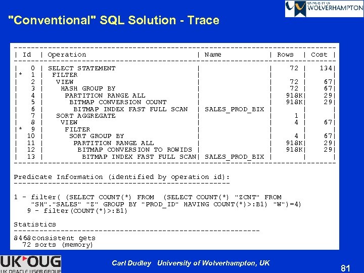 "Conventional" SQL Solution - Trace --------------------------------------| Id | Operation | Name | Rows | Cost | --------------------------------------| 0 | SELECT STATEMENT | 72 | 134| |* 1 | FILTER | | | | 2 | VIEW | 72 | 67| | 3 | HASH GROUP BY | 72 | 67| | 4 | PARTITION RANGE ALL | 918 K| 29| | 5 | BITMAP CONVERSION COUNT | 918 K| 29| | 6 | BITMAP INDEX FAST FULL SCAN | SALES_PROD_BIX | | | | 7 | SORT AGGREGATE | 1 | | | 8 | VIEW | 4 | 67| |* 9 | FILTER | | | | 10 | SORT GROUP BY | 4 | 67| | 11 | PARTITION RANGE ALL | 918 K| 29| | 12 | BITMAP CONVERSION TO ROWIDS | 918 K| 29| | 13 | BITMAP INDEX FAST FULL SCAN| SALES_PROD_BIX | | | --------------------------------------Predicate Information (identified by operation id): -------------------------1 - filter( (SELECT COUNT(*) FROM (SELECT COUNT(*) "ZCNT" FROM "SH". "SALES" "Z" GROUP BY "PROD_ID" HAVING COUNT(*)>: B 1) "W")=4) 9 - filter(COUNT(*)>: B 1) Statistics -----------------------------8468 consistent gets 72 sorts (memory) Carl Dudley University of Wolverhampton, UK 81
 nth Best Product – "Failed" SQL Solution Ø Find nth ranked product in terms of numbers of orders for each product SELECT prod_id , ycnt FROM (SELECT prod_id , COUNT(*) ycnt FROM sh. sales y GROUP BY prod_id) v WHERE &position - 1 = (SELECT COUNT(*) FROM (SELECT ycnt FROM v) w WHERE w. ycnt > v. ycnt); * ERROR at line 8: ORA-04044: procedure, function, package, or type is not allowed here Carl Dudley University of Wolverhampton, UK 82
 nth Best Product – Factored Subquery Solution Ø Find nth ranked product in terms of numbers of orders for each product WITH v AS (SELECT prod_id , COUNT(*) ycnt FROM sh. sales y GROUP BY prod_id) 5 SELECT prod_id , ycnt FROM v WHERE &position - 1 = (SELECT COUNT(*) FROM (SELECT ycnt FROM v) w WHERE w. ycnt > v. ycnt); PROD_ID YCNT --------- 33 22768 Elapsed: 00: 00. 07 Carl Dudley University of Wolverhampton, UK 83
 Factored Subquery Solution - Trace -------------------------------------------| Id | Operation | Name | Rows | Cost | -------------------------------------------| 0 | SELECT STATEMENT | | 1 | 71 | | 1 | TEMP TABLE TRANSFORMATION | | | | | 2 | LOAD AS SELECT | | | | 3 | HASH GROUP BY | 72 | 67 | | 4 | PARTITION RANGE ALL | 918 K| 29 | | 5 | BITMAP CONVERSION COUNT | | 918 K| 29 | | 6 | BITMAP INDEX FAST FULL SCAN| SALES_PROD_BIX | | | |* 7 | FILTER | | | | 8 | VIEW | 72 | | 9 | TABLE ACCESS FULL | SYS_TEMP_0 FD 9 D 661 A_14 D 8441 | 72 | | 10 | SORT AGGREGATE | 1 | | |* 11 | VIEW | 72 | | 12 | TABLE ACCESS FULL | SYS_TEMP_0 FD 9 D 661 A_14 D 8441 | 72 | -------------------------------------------Predicate Information (identified by operation id): ------------------------- 7 - filter( (SELECT COUNT(*) FROM (SELECT /*+ CACHE_TEMP_TABLE ("T 1") */ "C 0" "PROD_ID", "C 1" "YCNT" "SYS". "SYS_TEMP_0 FD 9 D 661 A_14 D 8441" "T 1") "V" WHERE "YCNT">: B 1)=4) 11 - filter("YCNT">: B 1) Statistics -----------------------------355 consistent gets 0 sorts (memory) Carl Dudley University of Wolverhampton, UK 84
 nth Best Product – Analytic Function Solution Ø Find nth ranked product in terms of numbers of orders for each product SELECT prod_id , vcnt FROM (SELECT prod_id , vcnt , RANK() OVER (ORDER BY vcnt DESC) rnk FROM (SELECT prod_id , COUNT(*) vcnt FROM sh. sales z GROUP BY z. prod_id)) qry 5 WHERE qry. rnk = &position; PROD_ID YCNT --------- 33 22768 Elapsed: 00: 00. 01 Carl Dudley University of Wolverhampton, UK 85
 Analytic Function Solution - Trace -------------------------------------| Id | Operation | Name | Rows | Cost | -------------------------------------| 0 | SELECT STATEMENT | 72 | 105| |* 1 | VIEW | 72 | 105| |* 2 | WINDOW SORT PUSHED RANK | 72 | 105| | 3 | HASH GROUP BY | 72 | 105| | 4 | PARTITION RANGE ALL | 918 K| 29| | 5 | BITMAP CONVERSION COUNT | 918 K| 29| | 6 | BITMAP INDEX FAST FULL SCAN| SALES_PROD_BIX | | | -------------------------------------Predicate Information (identified by operation id): ------------------------- 1 - filter("QRY". "RNK"=5) 2 - filter(RANK() OVER ( ORDER BY COUNT(*) DESC )<=5) Statistics -----------------------------116 consistent gets 1 sorts (memory) Carl Dudley University of Wolverhampton, UK 86
 Analytic Function Performance Ø Defining the PARTITION BY and ORDER BY clauses on indexed columns will provide optimum performance — For example, a composite index on (deptno, hiredate) columns will prove effective Ø Analytic functions still provide acceptable performance in absence of indexes but need to do sorting for computing based on partition and order by columns — If the query contains multiple analytic functions, sorting and partitioning on two different columns should be avoided if they are both not indexed Carl Dudley University of Wolverhampton, UK 87
") Performance Ø Hiding analytics in views can prevent the use of indexes — SUM(sal) has to be computed across all rows before the analysis CREATE OR REPLACE VIEW vv AS SELECT *, SUM(sal) OVER (PARTITION BY deptno) Deptno_Sum_Sal FROM emp; SELECT * FROM vv WHERE empno = 7900; EMPNO ENAME JOB MGR HIREDATE SAL COMM DEPTNO_SUM_SAL ----- ---- ------------- 7900 JAMES CLERK 7698 03 -DEC-81 950 30 9400 ----------------------| Id | Operation | Name | Rows | ----------------------| 0 | SELECT STATEMENT | | 14 | |* 1 | VIEW | VV | 14 | | 2 | WINDOW SORT | | 14 | | 3 | TABLE ACCESS FULL| EMP | 14 | ----------------------SELECT * FROM emp WHERE empno = 7900; ------------------------------| Id | Operation | Name | Rows | ------------------------------| 0 | SELECT STATEMENT | 1 | | 1 | TABLE ACCESS BY INDEX ROWID| EMP | 1 | |* 2 | INDEX UNIQUE SCAN | SYS_C 0017750 | 1 | ------------------------------Carl Dudley University of Wolverhampton, UK 88
Performance Ø Hiding analytics in views can prevent the use of indexes — SUM(sal) has to be computed across all rows before the analysis CREATE OR REPLACE VIEW vv AS SELECT *, SUM(sal) OVER (PARTITION BY deptno) Deptno_Sum_Sal FROM emp; SELECT * FROM vv WHERE empno = 7900; EMPNO ENAME JOB MGR HIREDATE SAL COMM DEPTNO_SUM_SAL ----- ---- ------------- 7900 JAMES CLERK 7698 03 -DEC-81 950 30 9400 ----------------------| Id | Operation | Name | Rows | ----------------------| 0 | SELECT STATEMENT | | 14 | |* 1 | VIEW | VV | 14 | | 2 | WINDOW SORT | | 14 | | 3 | TABLE ACCESS FULL| EMP | 14 | ----------------------SELECT * FROM emp WHERE empno = 7900; ------------------------------| Id | Operation | Name | Rows | ------------------------------| 0 | SELECT STATEMENT | 1 | | 1 | TABLE ACCESS BY INDEX ROWID| EMP | 1 | |* 2 | INDEX UNIQUE SCAN | SYS_C 0017750 | 1 | ------------------------------Carl Dudley University of Wolverhampton, UK 88
 OVER (PARTITION BY deptno ORDER") Steamy Windows SELECT empno, ename, sal, deptno , SUM(sal) OVER (PARTITION BY deptno ORDER BY sal) sumsal FROM emp ORDER BY deptno, sal; EMPNO ENAME SAL DEPTNO SUMSAL ---------- ----- 7934 MILLER 1300 10 1300 7782 CLARK 2450 10 3750 7839 KING 5000 10 8750 7369 SMITH 800 20 800 7876 ADAMS 1100 20 1900 7566 JONES 2975 20 4875 7788 SCOTT 3000 20 10875 7902 FORD 3000 20 10875 7900 JAMES 950 30 950 7654 MARTIN 1250 30 3450 7521 WARD 1250 30 3450 7844 TURNER 1500 30 4950 7499 ALLEN 1600 30 6550 7698 BLAKE 2850 30 9400 Default window is RANGE BETWEEN UNBOUNDED PRECEDING AND CURRENT ROW Carl Dudley University of Wolverhampton, UK 89
Steamy Windows SELECT empno, ename, sal, deptno , SUM(sal) OVER (PARTITION BY deptno ORDER BY sal) sumsal FROM emp ORDER BY deptno, sal; EMPNO ENAME SAL DEPTNO SUMSAL ---------- ----- 7934 MILLER 1300 10 1300 7782 CLARK 2450 10 3750 7839 KING 5000 10 8750 7369 SMITH 800 20 800 7876 ADAMS 1100 20 1900 7566 JONES 2975 20 4875 7788 SCOTT 3000 20 10875 7902 FORD 3000 20 10875 7900 JAMES 950 30 950 7654 MARTIN 1250 30 3450 7521 WARD 1250 30 3450 7844 TURNER 1500 30 4950 7499 ALLEN 1600 30 6550 7698 BLAKE 2850 30 9400 Default window is RANGE BETWEEN UNBOUNDED PRECEDING AND CURRENT ROW Carl Dudley University of Wolverhampton, UK 89
 SELECT empno, ename, sal, deptno , SUM(sal) OVER (PARTITION BY deptno") Steamy Windows (continued) SELECT empno, ename, sal, deptno , SUM(sal) OVER (PARTITION BY deptno ORDER BY sal) sumsal FROM emp WHERE ename LIKE '%M%' ORDER BY deptno , sal EMPNO ENAME SAL DEPTNO SUMSAL ---------- ----- 7934 MILLER 1300 10 1300 7369 SMITH 800 20 800 7876 ADAMS 1100 20 1900 7900 JAMES 950 30 950 7654 MARTIN 1250 30 2200 SELECT * FROM (SELECT empno, ename, sal, deptno , SUM(sal) OVER (PARTITION BY deptno ORDER BY sal) sumsal FROM emp ) Includes WARD who is in department 30 WHERE ename LIKE '%M%' and has a salary of 1250. which is within ORDER BY deptno , sal; the RANGE with MARTIN EMPNO ENAME SAL DEPTNO SUMSAL ---------- ----- 7934 MILLER 1300 10 1300 7369 SMITH 800 20 800 7876 ADAMS 1100 20 1900 7900 JAMES 950 30 950 7654 MARTIN 1250 30 3450 Carl Dudley University of Wolverhampton, UK 90
Steamy Windows (continued) SELECT empno, ename, sal, deptno , SUM(sal) OVER (PARTITION BY deptno ORDER BY sal) sumsal FROM emp WHERE ename LIKE '%M%' ORDER BY deptno , sal EMPNO ENAME SAL DEPTNO SUMSAL ---------- ----- 7934 MILLER 1300 10 1300 7369 SMITH 800 20 800 7876 ADAMS 1100 20 1900 7900 JAMES 950 30 950 7654 MARTIN 1250 30 2200 SELECT * FROM (SELECT empno, ename, sal, deptno , SUM(sal) OVER (PARTITION BY deptno ORDER BY sal) sumsal FROM emp ) Includes WARD who is in department 30 WHERE ename LIKE '%M%' and has a salary of 1250. which is within ORDER BY deptno , sal; the RANGE with MARTIN EMPNO ENAME SAL DEPTNO SUMSAL ---------- ----- 7934 MILLER 1300 10 1300 7369 SMITH 800 20 800 7876 ADAMS 1100 20 1900 7900 JAMES 950 30 950 7654 MARTIN 1250 30 3450 Carl Dudley University of Wolverhampton, UK 90
 In the Final Analysis So we have discussed Ø The ranking of data using analytic functions Ø Partitioning datasets from queries Ø Using aggregate functions in analytic scenarios Ø How to apply sliding windows to query results Ø Comparing values across rows Ø Performance characteristics Carl Dudley University of Wolverhampton, UK 91
 Analytic Functions Carl Dudley University of Wolverhampton, UK UKOUG Council Oracle ACE Director carl. dudley@wlv. ac. uk Carl Dudley University of Wolverhampton, UK 92