Analytical Tools Marginal analysis Discounted cash flow

Analytical Tools Marginal analysis Discounted cash flow

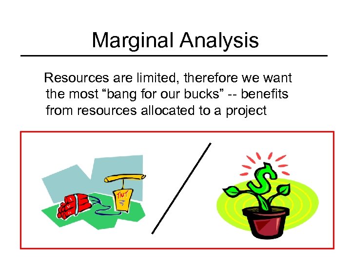Marginal Analysis Resources are limited, therefore we want the most “bang for our bucks” -- benefits from resources allocated to a project

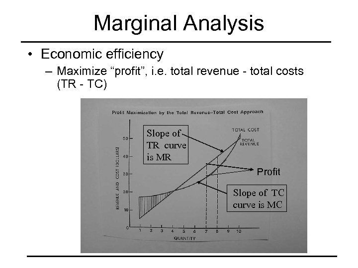Marginal Analysis • Economic efficiency – Maximize “profit”, i. e. total revenue - total costs (TR - TC) Slope of TR curve is MR Profit Slope of TC curve is MC

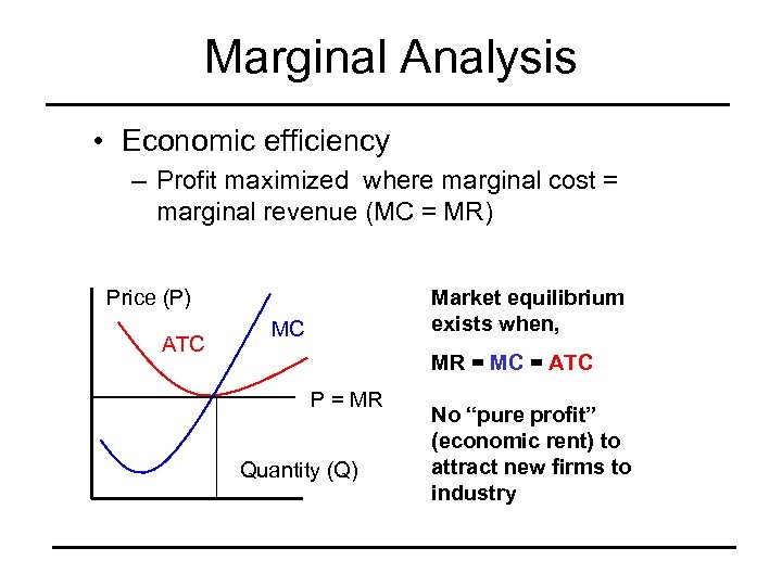Marginal Analysis • Economic efficiency – Profit maximized where marginal cost = marginal revenue (MC = MR) Price (P) ATC Market equilibrium exists when, MC MR = MC = ATC P = MR Quantity (Q) No “pure profit” (economic rent) to attract new firms to industry

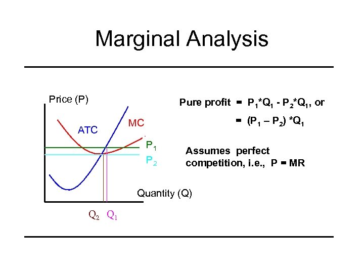Marginal Analysis Price (P) Pure profit = P 1*Q 1 - P 2*Q 1, or ATC = (P 1 – P 2) *Q 1 MC P 1 P 2 Assumes perfect competition, i. e. , P = MR Quantity (Q) Q 2 Q 1

Advantage of Marginal Analysis • Don’t have to do a complete analysis of costs and revenues • Can estimate MC directly from market price by assuming a given profit percentage • Can estimate MR from market price and knowledge of market structure, i. e. perfectly competitive, monopolistic, or somewhere inbetween.

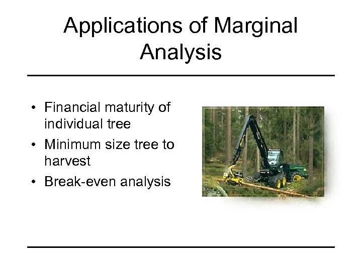Applications of Marginal Analysis • Financial maturity of individual tree • Minimum size tree to harvest • Break-even analysis

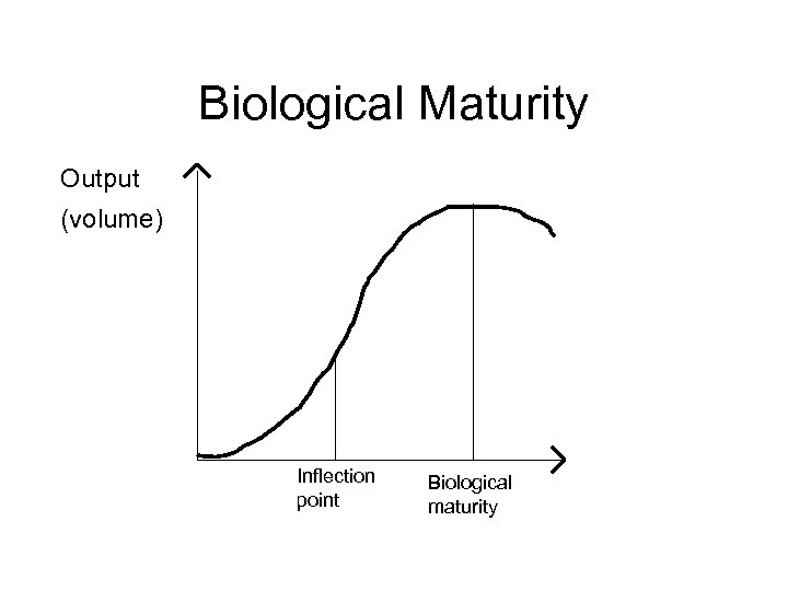Biological Maturity Output (volume) Inflection point Biological maturity

Biological vs. Financial Maturity • Financial maturity is based on benefit from letting tree/stand grow for another time period compared to cost for doing so. • Would you expect biological and financial maturity to occur at the same point in time?

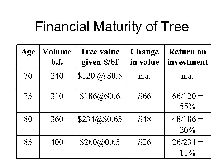Financial Maturity of Tree Age Volume b. f. Tree value given $/bf Change Return on in value investment 70 240 $120 @ $0. 5 n. a. 75 310 $186@$0. 6 $66 80 360 $234@$0. 65 $48 85 400 $260@0. 65 $26 66/120 = 55% 48/186 = 26% 26/234 = 11%

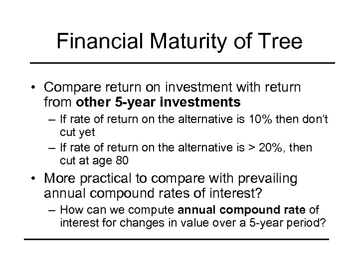Financial Maturity of Tree • Compare return on investment with return from other 5 -year investments – If rate of return on the alternative is 10% then don’t cut yet – If rate of return on the alternative is > 20%, then cut at age 80 • More practical to compare with prevailing annual compound rates of interest? – How can we compute annual compound rate of interest for changes in value over a 5 -year period?

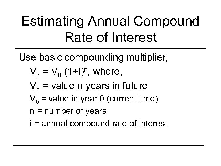Estimating Annual Compound Rate of Interest Use basic compounding multiplier, Vn = V 0 (1+i)n, where, Vn = value n years in future V 0 = value in year 0 (current time) n = number of years i = annual compound rate of interest

Before solving for I let’s review how compounding and discounting multipliers are used

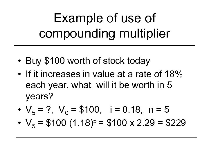Example of use of compounding multiplier • Buy $100 worth of stock today • If it increases in value at a rate of 18% each year, what will it be worth in 5 years? • V 5 = ? , V 0 = $100, i = 0. 18, n = 5 • V 5 = $100 (1. 18)5 = $100 x 2. 29 = $229

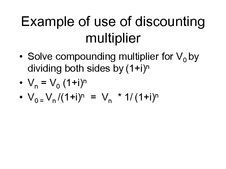Example of use of discounting multiplier • Solve compounding multiplier for V 0 by dividing both sides by (1+i)n • Vn = V 0 (1+i)n • V 0 = Vn /(1+i)n = Vn * 1/ (1+i)n

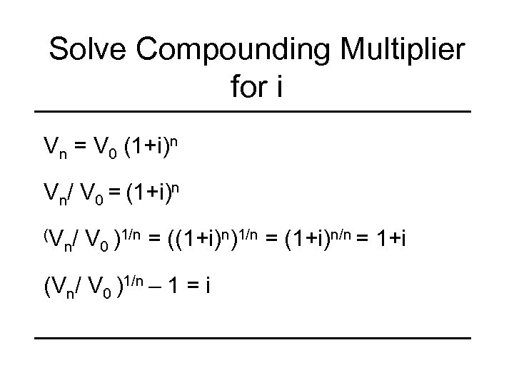Solve Compounding Multiplier for i Vn = V 0 (1+i)n Vn/ V 0 = (1+i)n (V / V 0 )1/n = ((1+i)n)1/n = (1+i)n/n = 1+i n (Vn/ V 0 )1/n – 1 = i

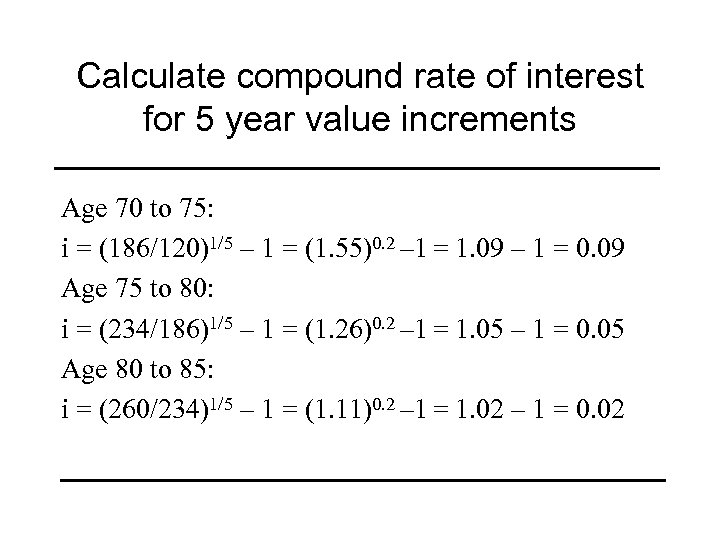Calculate compound rate of interest for 5 year value increments Age 70 to 75: i = (186/120)1/5 – 1 = (1. 55)0. 2 – 1 = 1. 09 – 1 = 0. 09 Age 75 to 80: i = (234/186)1/5 – 1 = (1. 26)0. 2 – 1 = 1. 05 – 1 = 0. 05 Age 80 to 85: i = (260/234)1/5 – 1 = (1. 11)0. 2 – 1 = 1. 02 – 1 = 0. 02

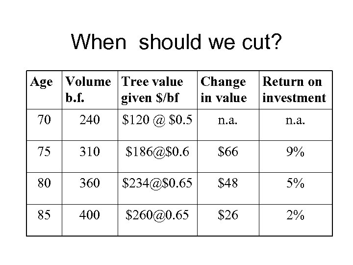When should we cut? Age Volume Tree value b. f. given $/bf Change in value Return on investment 70 240 $120 @ $0. 5 n. a. 75 310 $186@$0. 6 $66 9% 80 360 $234@$0. 65 $48 5% 85 400 $260@0. 65 $26 2%

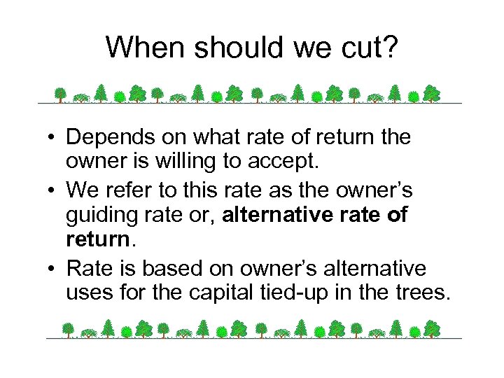When should we cut? • Depends on what rate of return the owner is willing to accept. • We refer to this rate as the owner’s guiding rate or, alternative rate of return. • Rate is based on owner’s alternative uses for the capital tied-up in the trees.

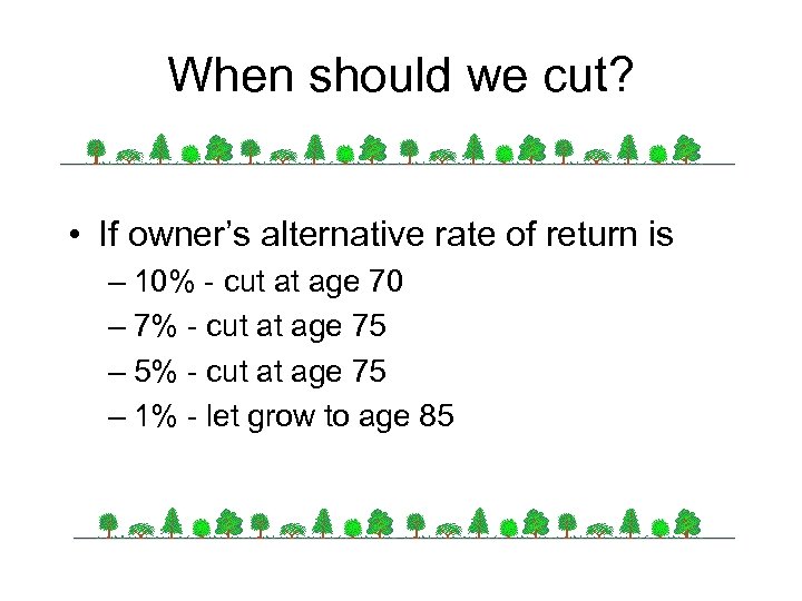When should we cut? • If owner’s alternative rate of return is – 10% - cut at age 70 – 7% - cut at age 75 – 5% - cut at age 75 – 1% - let grow to age 85

How does an owner select her alternative rate of return? • Borrowing rate – if she would have to borrow money if tree wasn’t get, she could use the interest rate she would have to pay on the loan, i. e. the “borrowing rate” • Lending rate – if owner could “lend” the revenue from cutting the tree now to someone else, she could use the rate she would get by making the “loan”

Minimum Size Tree to Cut Logger buys cutting rights on 200 acre tract of pine pulpwood for lump sum amount of $40, 000. Landowner placed no limits on what logger can cut. Logger wants to cut to maximize net revenue (profit). Should he give cutting crew a minimum size tree to cut? Answer with marginal approach.

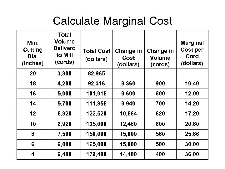Calculate Marginal Cost Min. Cutting Dia. (inches) Total Volume Deliverd to Mill (cords) 20 3, 300 82, 965 18 4, 200 92, 316 9, 360 900 10. 40 16 5, 000 101, 916 9, 600 800 12. 00 14 5, 700 111, 856 9, 940 700 14. 20 12 6, 320 122, 520 10, 664 620 17. 20 10 6, 920 135, 000 12, 480 600 20. 80 8 7, 500 150, 000 15, 000 580 25. 86 6 8, 000 165, 000 15, 000 500 30. 00 4 8, 400 179, 400 14, 400 36. 00 Total Cost Change in Cost Volume (dollars) (cords) Marginal Cost per Cord (dollars)

Compare MC and MB • If price per cord received by logger is $30, then shouldn’t cut any tree less than about 7 inches. • If price per cord increases to $35, then cut down to 5 inches. • If price per cord decreases to $25, then cut down to about 9 inches

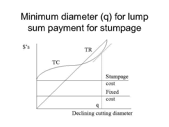Minimum diameter (q) for lump sum payment for stumpage $’s TR TC Stumpage cost Fixed cost q Declining cutting diameter

Pay as cut contract • Would minimum diameter change if logger paid for stumpage as trees were cut (log scale) instead of for lump sum amount in advance? • Yes, stumpage now a variable cost, not a fixed cost

Analytical Tools • Discounted cash flow – Net present value • Discount or compound all cash flows to same point in time • Calculate using an assumed interest rate – Internal rate of return • Interest rate (i) that makes NPV zero, i. e. equates PV of all costs and all benefits • “Calculate” the interest rate

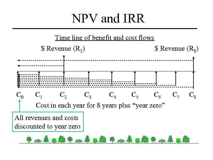NPV and IRR Time line of benefit and cost flows $ Revenue (R 2) C 0 $ Revenue (R 8) C 1 C 2 C 3 C 4 C 5 C 6 Cost in each year for 8 years plus “year zero” All revenues and costs discounted to year zero C 7 C 8

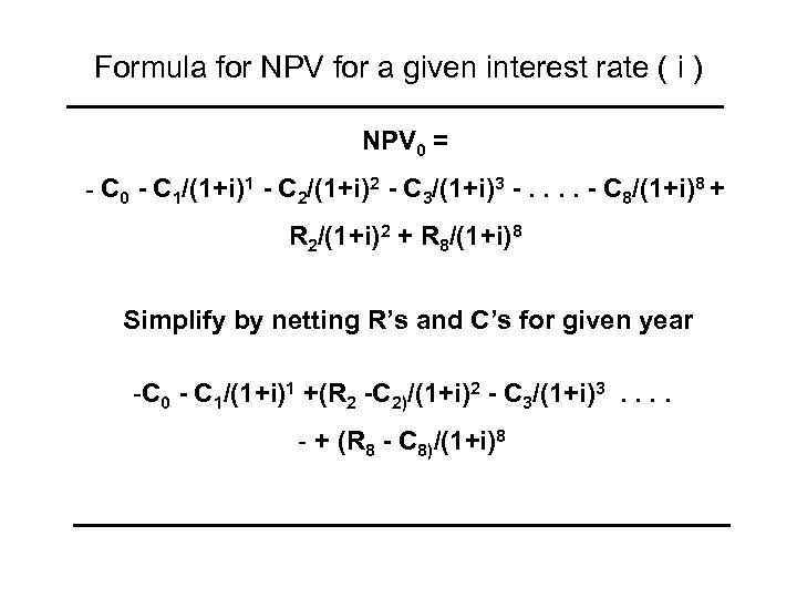Formula for NPV for a given interest rate ( i ) NPV 0 = - C 0 - C 1/(1+i)1 - C 2/(1+i)2 - C 3/(1+i)3 -. . - C 8/(1+i)8 + R 2/(1+i)2 + R 8/(1+i)8 Simplify by netting R’s and C’s for given year -C 0 - C 1/(1+i)1 +(R 2 -C 2)/(1+i)2 - C 3/(1+i)3. . - + (R 8 - C 8)/(1+i)8

NPV Using Summation Notation n NPV = where, [ (Rt – Ct)/(1+i)t] t=0 NPV = unknown n = number of years Rt = revenue (income) in year t Ct = cost (expense) in year t t = index number for years i = discount rate (alternative rate of return)

Internal Rate of Return Using Summation Notation n NPV = [ (Rt – Ct)/(1+i)t] t=1 where, NPV = 0 Rt = revenue (income) in year t Ct = expense (cost) in year t t = index number for years i = unknown

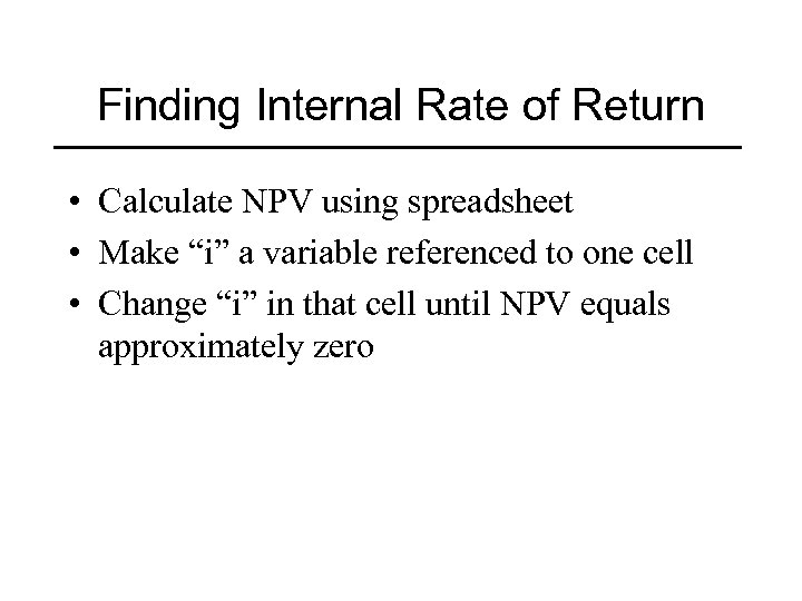Finding Internal Rate of Return • Calculate NPV using spreadsheet • Make “i” a variable referenced to one cell • Change “i” in that cell until NPV equals approximately zero