An Experimental Comparison of Posted Prices with Single-Buyer

An Experimental Comparison of Posted Prices with Single-Buyer and Multi-Buyer Prices Nejat Anbarci Deakin University and Nick Feltovich Monash University

Search models in economics The concept of search has been a versatile one in economic theory. - Price dispersion in goods markets (Salop and Stiglitz, 1977 REStud; Burdett and Judd, 1983 Econometrica) - Unemployment and job vacancies (Pissarides, 1985 AER) - Money as a medium of exchange (Kiyotaki and Wright, 1989 JPE; 1993 AER) - Discrimination by consumers or firms (Borjas and Bronars, 1989 JPE; Black, 1995 JLabor. Econ) The 2010 Nobel Prize in Economics was awarded to three leading search theorists, Diamond, Mortensen and Pissarides, who laid the foundations of the above applied work.

Random vs directed search Much early work on search assumed that search is undirected or random: an agent on one side of the market is likely to meet any of the agents on the other side with a matching probability. This approach has been innovative, but has faced criticisms: “[i]n contrast to what happens in search models, exchanges in actual market economies are organized by specialist traders, who mitigate search costs by providing facilities that are easy to locate. Thus, when people wish to buy shoes they go to a shoe store; when hungry they go to a grocer; when desiring to sell their labor services they go to firms known to offer employment” (Howitt, 2005 IER, p. 405). The solution is not to dispense with search altogether, but to look at directed instead of undirected search. (Buyers choose which seller(s) to visit, based on some relevant information. )

Bargaining and posted prices: historically and now Much early work on search also assumed bargaining alongside with random search. Bargaining was the predominant trading protocol in markets throughout the world until the early 19 th century. The use of posted prices is a relatively recent phenomenon. Its ascent and eventual widespread use date back to 1823 when Alexander Stewart introduced posted prices in his NYC ‘Marble Dry Goods Palace’, which grew to become the largest in the U. S. Other famous merchants followed his lead. Currently, bargaining and posted prices co-exist as common means of establishing prices universally - e. g. , housing/second-hand car prices vs supermarket prices (Anbarci and Gomis-Porqueras, 2012: a dynamic model with co-existing bargaining and price-posting firms, using replicator dynamics; Anbarci, Dutu & Sun, 2012: use of bargaining and price-posting in the LW (2005 JPE) setup but with “production in advance” instead of “production on demand”).

Uninformed buyers: bargaining vs posted prices Diamond (1987 The New Palgrave, 279) noted that in actual markets “infrequent traders are often ill-informed. . . [creating an incentive for] sellers to find consumers whose beliefs make them willing to trade at high prices. ” Similarly, Stigler (1961 JPE, 218 -19) noted the “widely held view that inexperienced buyers (tourists) pay higher prices than do experienced buyers. ” Macy’s advertisements from the 1850 s stated that prior to the use of posted prices (by Macy’s), “there was no regular price for anything and the most ignorant were the most imposed upon, ” while with posted prices “a child can trade with us as cheap as the shrewdest buyer in the country” (Scull, 1967)

The BWS setup Burdett, Shi and Wright (2001 JPE) considered a market with posted prices and directed search (recall that bargaining with random search was the main paradigm in many earlier search papers). In the simple version of their model: - One homogeneous indivisible good. - Two identical firms; each can produce up to one unit of the good at 0 cost. - Two identical buyers, each valuing the first unit of the good at 1; no benefit from additional units. - Sellers simultaneously post prices; these are observed by buyers, who simultaneously choose which seller to visit. - Random buyer chosen to buy, from all visiting the same seller; for the empty-handed buyer, visiting the empty-handed seller is prohibitively costly.

BSW results BSW show that a large number of subgame-perfect equilibria exists. They impose additional symmetry and robustness criteria, and find a unique equilibrium: both sellers choose p = 0. 5 and are visited with equal probability by a given buyer. → Frictions are possible, even though there is complete information about firms’ prices, capacities and locations. (Taking limits doesn’t help with infinite replicas of buyers and sellers. ) There are (coordinated) pure-strategy equilibria as well: “Buyer 1 visiting Seller 1 and Buyer 2 visiting Seller 2”, “Buyer 1 visiting Seller 2 and Buyer 2 visiting Seller 1”, which are efficient. There is a large range of asymmetric seller prices supporting these pure -strategy equilibria.

The CE setup and result Coles and Eeckhout (2003 JET) note that posted-price models such as BSW’s ignore the market power sellers have when visited by more buyers than their capacity. They argue that these models should allow posting of prices that are contingent on demand to benefit sellers. Their simple model is like BSW’s, except sellers simultaneously post “schedules” of prices: a one-buyer price and a multibuyer price. CE show that under some assumptions, equilibria are very similar to those in BSW’s model. Both sellers still choose p 1 = 0. 5 and are visited with equal probability by a given buyer, but p 2 is indeterminate in [0, 1] (though equal for the two sellers).

Some misgivings about BSW and CE setups CE remark that while setting high multi-buyer prices ought to be profit enhancing, “in many [field] environments such opportunistic behavior is not observed” (p. 266), due possibly to repeated-game effects. BSW’s and CE’s results depend on selection criteria - such as on symmetry - that may or may not be reasonable (some buyers may visit the seller with the higher price to make sure that they receive the good for sure). Without such criteria, there is a large number of equilibria. The additional flexibility of demand-contingent multi-buyer pricing of CE may not unambiguously benefit sellers contrary to CE’s claim (e. g. , sellers may post lower multi-buyer prices to lure all buyers).

Theoretical predictions of BSW and CE setups To shed some light on how these posted pricing institutions affect market outcomes, we conduct an experiment that implements the BSW and CE models, with minor changes. Buyer values are 20 and seller costs are 10; seller cost is avoidable (production on demand). Theoretical predictions (from BSW, CE arguments): - BSW price = CE one-buyer price = 15. - CE two-buyer price is indeterminate (but equal for both sellers in a market). - Each buyer/seller has a 0. 75 chance of trading. - Surpluses shared equally between buyers and sellers in BSW. Indeterminate in CE - supposedly higher surplus going to sellers.

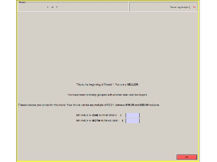
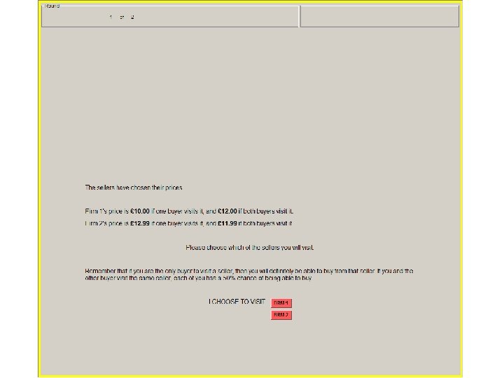
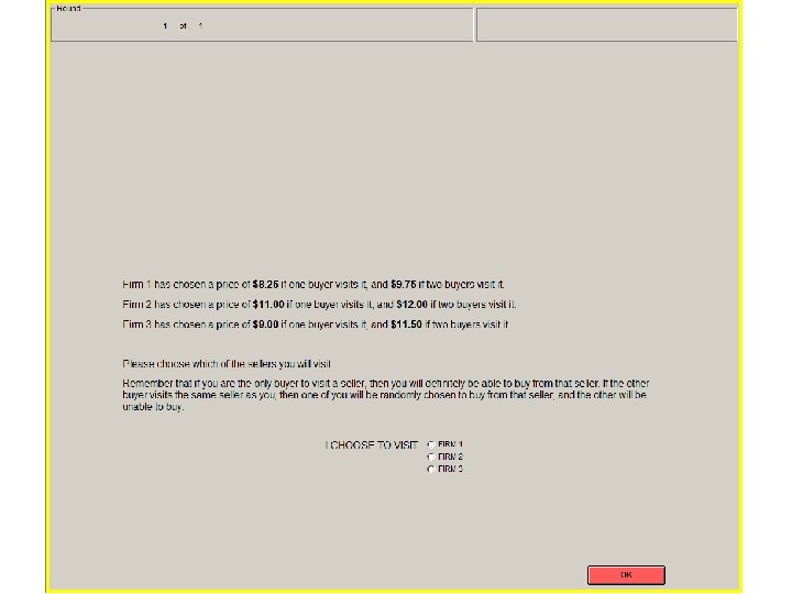
The BSW/CE 2 x 2 experiment - The experiment took place at SEEL (University of Aberdeen, Scotland); subjects were undergraduates and post-graduates from many programmes. Recruitment by ORSEE (Greiner, 2004). - Interaction via z-Tree (Fischbacher, 2007 Exp. Econ), with partitions preventing viewing of others’ screens. No identifying information about other subjects given. - Subjects played 20 rounds of the BSW game and 20 of the CE game (counterbalanced – 64 subjects in each ordering), with relevant instructions read before game starts.

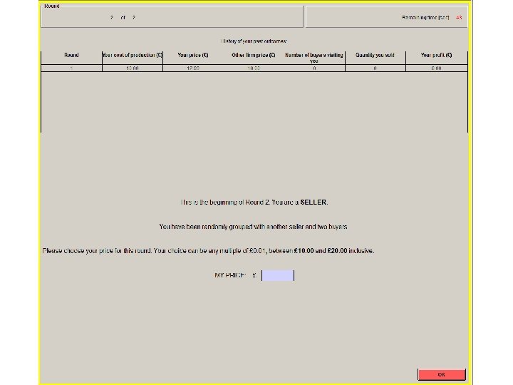
The BSW/CE 2 x 2 experiment (cont. d) - Roles fixed for entire session, but group compositions changed from round to round. - Prices restricted to multiples of £ 0. 01, between £ 10 and £ 20 (£ 1 ≈ 1. 5 -1. 6 AUD). - Sellers explicitly told in CE game that p 2 could be greater than, less than or equal to p 1. - Sellers were given “Firm 1”/“Firm 2” labels on buyers’ screens (i. i. d. across rounds).

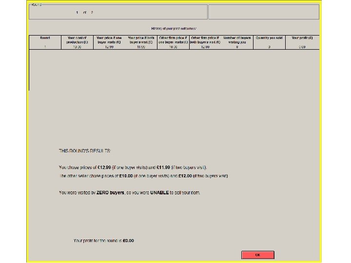
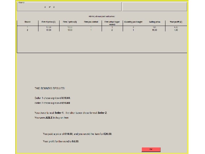
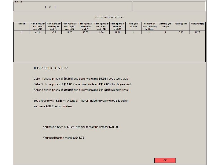
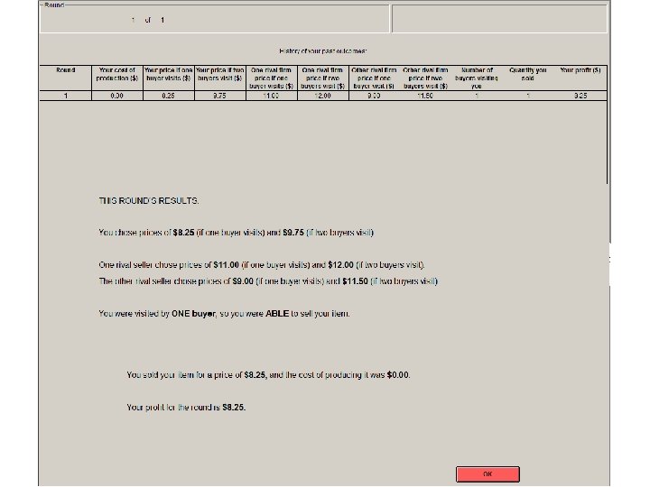
The BSW/CE 2 x 2 experiment (cont. d) - End-of-round feedback (also in history table): Sellers: own/opponent’s price, number of buyers visiting, quantity, profit. Buyers: seller prices, buyers’ visit choices, quantity, profit. - Subjects were paid (exactly) the sum of their profits from 4 randomly chosen rounds. - Average payoffs were roughly £ 20 (including a £ 3 show-up fee); sessions averaged 60 minutes.

Experimental design and procedures

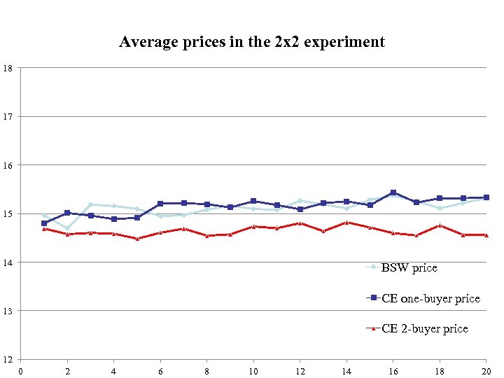
Average prices in the 2 x 2 experiment 18 17 16 15 14 BSW price CE one-buyer price 13 CE 2 -buyer price 12 0 2 4 6 8 10 12 14 16 18 20

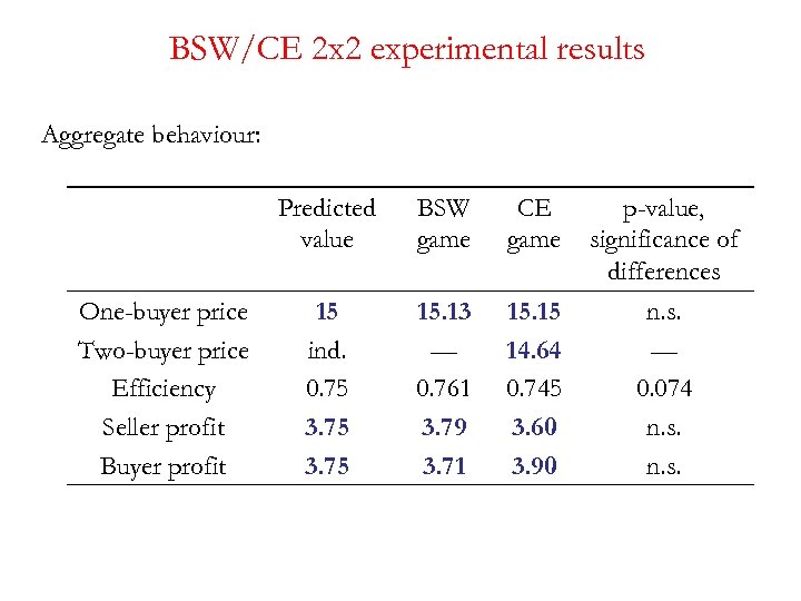
BSW/CE 2 x 2 experimental results Aggregate behaviour: Predicted value One-buyer price Two-buyer price Efficiency Seller profit Buyer profit BSW game CE game 15 ind. 0. 75 3. 75 15. 13 — 0. 761 3. 79 3. 71 15. 15 14. 64 0. 745 3. 60 3. 90 p-value, significance of differences n. s. — 0. 074 n. s.

BSW/CE 2 x 2 experimental results (cont. d) Other significance results: - Two-buyer prices in CE marginally significantly less than onebuyer prices in CE (p ≈ 0. 055). - Two-buyer prices in CE significantly less than prices in BSW (p ≈ 0. 007).

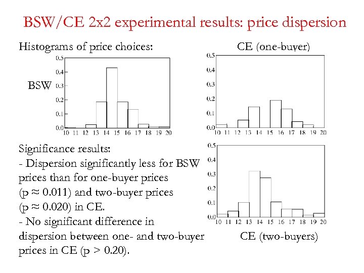
BSW/CE 2 x 2 experimental results: price dispersion Histograms of price choices: CE (one-buyer) BSW Significance results: - Dispersion significantly less for BSW prices than for one-buyer prices (p ≈ 0. 011) and two-buyer prices (p ≈ 0. 020) in CE. - No significant difference in dispersion between one- and two-buyer prices in CE (p > 0. 20). CE (two-buyers)

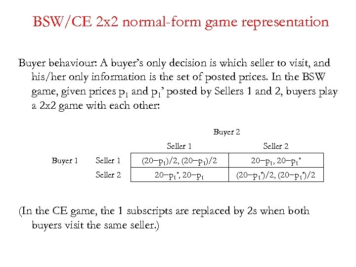
BSW/CE 2 x 2 normal-form game representation Buyer behaviour: A buyer’s only decision is which seller to visit, and his/her only information is the set of posted prices. In the BSW game, given prices p 1 and p 1’ posted by Sellers 1 and 2, buyers play a 2 x 2 game with each other: Buyer 2 Seller 1 (20−p 1)/2, (20−p 1)/2 20−p 1, 20−p 1’ Seller 2 Buyer 1 Seller 2 20−p 1’, 20−p 1 (20−p 1’)/2, (20−p 1’)/2 (In the CE game, the 1 subscripts are replaced by 2 s when both buyers visit the same seller. )

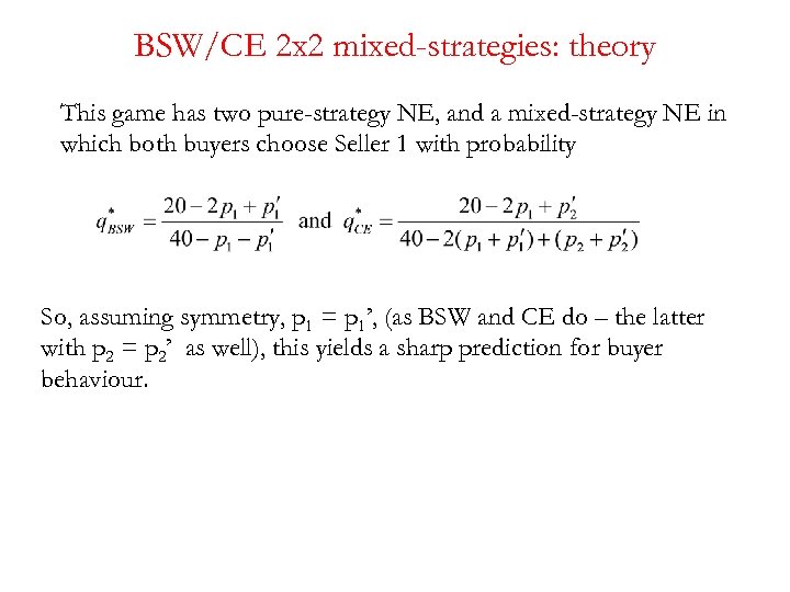
BSW/CE 2 x 2 mixed-strategies: theory This game has two pure-strategy NE, and a mixed-strategy NE in which both buyers choose Seller 1 with probability So, assuming symmetry, p 1 = p 1’, (as BSW and CE do – the latter with p 2 = p 2’ as well), this yields a sharp prediction for buyer behaviour.

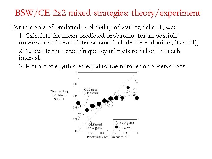
BSW/CE 2 x 2 mixed-strategies: theory/experiment For intervals of predicted probability of visiting Seller 1, we: 1. Calculate the mean predicted probability for all possible observations in each interval (and include the endpoints, 0 and 1); 2. Calculate the actual frequency of visits to Seller 1 in each interval; 3. Plot a circle with area equal to the number of observations.

The BSW/CE 3 x 2/2 x 3 follow-up experiment The 2 (buyers) x 2 (sellers) setup is the simplest non-trivial version of this kind of market, and is the one analysed in most detail by BSW and CE (and others). However, the 2 x 2 setup is a bit mundane (if not boring)! As a follow-up, we consider the asymmetric 3 x 2 and 2 x 3 setups. The experiment is taking place at Mon. LEE (still in progress).

What is different in the BSW/CE 3 x 2/2 x 3 setups? As before: - End-of-round feedback (also in history table): Sellers: own/opponent’s price, number of buyers visiting, quantity, profit. Buyers: seller prices, number of buyers visiting same seller, quantity, profit. Minor changes: - Prices restricted to multiples of $0. 05, between 0 and $20. - Subjects were paid according to the results from 6 randomly chosen rounds. - Average payoffs were roughly $20 for the unfavoured side of the market, $60 for the favoured side (incl. $10 show-up fee).

Theoretical predictions: BSW/CE 3 x 2/2 x 3 setups Theoretical predictions (vs core/auctions predictions - odd-man out): 3 x 2 game - BSW price = CE one-buyer price ≈ 14. 55. - CE multi-buyer price is indeterminate (but equal for both sellers in a market). - Each buyer has a 0. 583 chance of buying; each seller has a 0. 875 chance of selling. 2 x 3 game - BSW price = CE one-buyer price ≈ 5. 45. - CE multi-buyer price is indeterminate (but equal for both sellers in a market). - Each buyer has a 0. 833 chance of buying; each seller has a 0. 556 chance of selling.

Experimental design and procedures

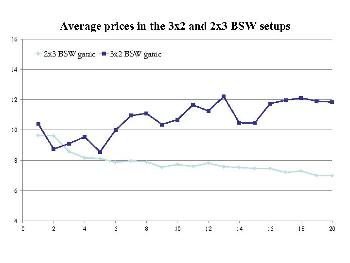
Average prices in the 3 x 2 and 2 x 3 BSW setups 16 2 x 3 BSW game 3 x 2 BSW game 14 12 10 8 6 4 0 2 4 6 8 10 12 14 16 18 20

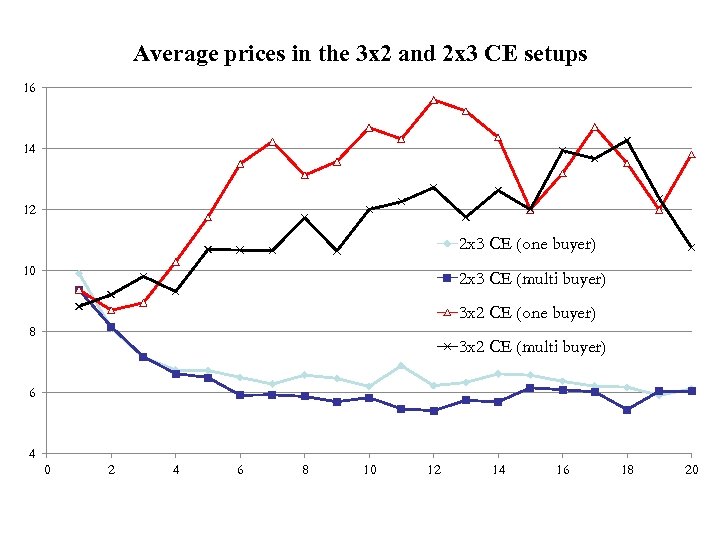
Average prices in the 3 x 2 and 2 x 3 CE setups 16 14 12 2 x 3 CE (one buyer) 10 2 x 3 CE (multi buyer) 3 x 2 CE (one buyer) 8 3 x 2 CE (multi buyer) 6 4 0 2 4 6 8 10 12 14 16 18 20

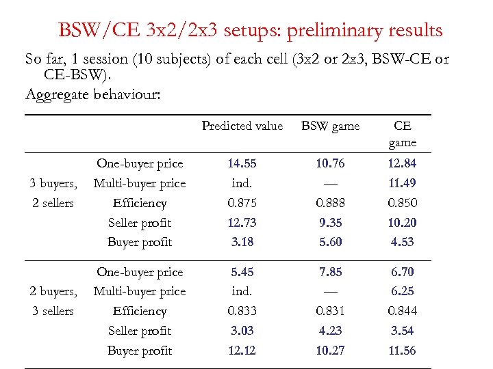
BSW/CE 3 x 2/2 x 3 setups: preliminary results So far, 1 session (10 subjects) of each cell (3 x 2 or 2 x 3, BSW-CE or CE-BSW). Aggregate behaviour: Predicted value 3 buyers, 2 sellers 2 buyers, 3 sellers BSW game CE game One-buyer price Multi-buyer price Efficiency Seller profit Buyer profit 14. 55 ind. 0. 875 12. 73 3. 18 10. 76 — 0. 888 9. 35 5. 60 12. 84 11. 49 0. 850 10. 20 4. 53 One-buyer price Multi-buyer price Efficiency Seller profit Buyer profit 5. 45 ind. 0. 833 3. 03 12. 12 7. 85 — 0. 831 4. 23 10. 27 6. 70 6. 25 0. 844 3. 54 11. 56

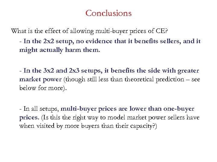
Conclusions What is the effect of allowing multi-buyer prices of CE? - In the 2 x 2 setup, no evidence that it benefits sellers, and it might actually harm them. - In the 3 x 2 and 2 x 3 setups, it benefits the side with greater market power (though still less than theoretical prediction – see below for more). - In all setups, multi-buyer prices are lower than one-buyer prices. (Is this the right way to model market power sellers have when visited by more buyers than their capacity? )

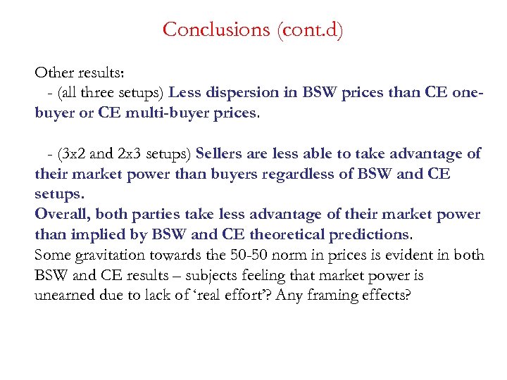
Conclusions (cont. d) Other results: - (all three setups) Less dispersion in BSW prices than CE onebuyer or CE multi-buyer prices. - (3 x 2 and 2 x 3 setups) Sellers are less able to take advantage of their market power than buyers regardless of BSW and CE setups. Overall, both parties take less advantage of their market power than implied by BSW and CE theoretical predictions. Some gravitation towards the 50 -50 norm in prices is evident in both BSW and CE results – subjects feeling that market power is unearned due to lack of ‘real effort’? Any framing effects?

Next step? - Add ‘costly’ money to this setting. Joint project with Nick and Richard Dutu (Deakin University, Graduate School of Business). Capture inflation by requiring buyers to borrow before visiting a seller. How does the inflation rate influence market outcomes? Main prediction: CE 2 -buyer price indeterminacy will disappear with any positive inflation/nominal interest rate (i. e. , with any level of cost of using money). Another (more mundane) prediction: Prices posted by sellers will be lower the higher the inflation/nominal interest rates. So far, some 2 x 2 sessions have been completed (see the preview). Next, we will run a few more 2 x 2 sessions and a significant number of 3 x 2, 2 x 3 sessions.

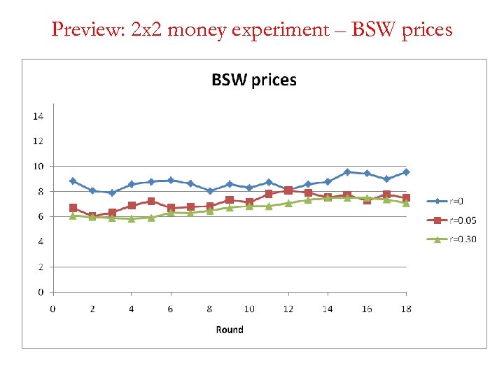
Preview: 2 x 2 money experiment – BSW prices

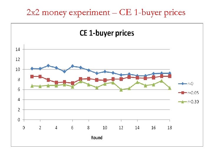
2 x 2 money experiment – CE 1 -buyer prices

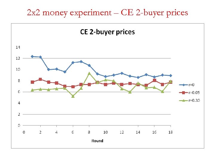
2 x 2 money experiment – CE 2 -buyer prices