Ammonia Toxicity Model AMMTOX Training Session Held 5

Ammonia Toxicity Model AMMTOX Training Session Held 5 Dec 2005 Hosted by EPA Region VIII Presented by Jim Saunders, Colorado WQCD

Purpose of Training Session • Explain rationale for model • Identify data needs and sources, including options for use of site-specific data • Demonstrate operation of model • Work with test data sets

Assumptions and Disclaimers • • Familiarity with Excel is assumed VB programming is NOT covered Future tech support is not my job Merits of National Criteria are not open for discussion • Ideas and suggestions presented in this session may not conform to policies of state or federal permitting agencies

Section 1: Concepts and Construction Central Question: Where is there greatest risk of exceeding stream standard? Depends on pollutant behavior and control of toxicity

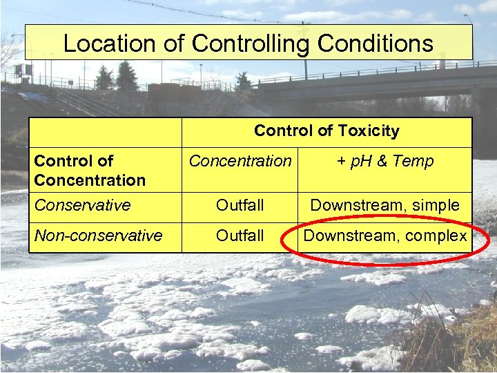Location of Controlling Conditions Control of Toxicity Control of Concentration + p. H & Temp Conservative Outfall Downstream, simple Non-conservative Outfall Downstream, complex

How do you handle a problem like Ammonia? • Calculating permit limits becomes difficult when controlling conditions are displaced downstream • Good news: solution likely to benefit discharger

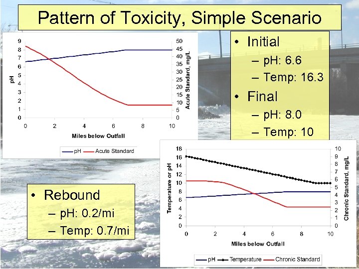Pattern of Toxicity, Simple Scenario • Initial – p. H: 6. 6 – Temp: 16. 3 • Final – p. H: 8. 0 – Temp: 10 • Rebound – p. H: 0. 2/mi – Temp: 0. 7/mi

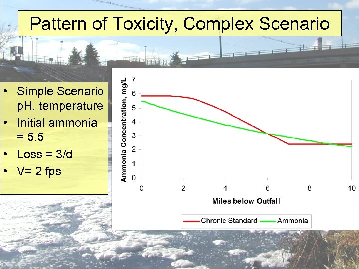Pattern of Toxicity, Complex Scenario • Simple Scenario p. H, temperature • Initial ammonia = 5. 5 • Loss = 3/d • V= 2 fps

Required Tasks • Define d/s trajectory of stream standard • Define d/s trajectory of ammonia concentration • Determine maximum effluent concentration such that instream ammonia will not exceed standard at any point downstream

Trajectory of Standard • Effect of effluent on stream chemistry generally elevates standard • Effect is transitory • Initial value of standard declines downstream because underlying controls (p. H and temperature) trend separately toward “equilibrium” values • Greatest risk of exceedance may occur anywhere between outfall and equilibrium conditions

What is equilibrium? • Stable p. H and temperature characteristic of this mixture of effluent and stream water • May differ from upstream conditions, especially if effluent flow is large • Equilibrium is dynamic with substantial diel and seasonal variation in p. H and temperature • This variability must be captured in standard

Trajectories for p. H and Temperature • Initial mixed conditions defined from flowweighted mean p. H and temperature • Effect of effluent on stream p. H and temperature is transitory • Initial mixed p. H and temperature trend separately toward “equilibrium” values • If the equilibrium value and the rate of change are known, p. H or temperature can be predicted at any point downstream of the outfall

Setpoint: Equilibrium with Regulatory Twist • p. H and temperature associated with greatest risk of exceeding ammonia standard for equilibrium conditions • Worst case in each month, subject to once -in-three-year exceedance • Terminus for p. H and temperature trajectories, not a fixed location

Why Obtaining Setpoint is Difficult • Sole task of Recur model • Field grab samples form framework • Apply characteristics of temporal variation to construct set of hourly values spanning entire period of record • Calculate standards hourly and determine acute (1 -h) and chronic (30 -d) values consistent with once-in-three-year exceedance threshold • Find associated p. H (acute and chronic) and temperature (chronic)

Application for Setpoint • Hidden hand – guides p. H and temperature toward target with regulatory meaning • Essential for producing d/s trajectory of ammonia standard, separately for acute and chronic

Back up a step. . Incorporation of temporal variation • p. H and temperature in stream exhibit temporal variation of diel and seasonal scales. . . thus applies to standard, too • Predictable diel pattern – Based on sine curve – Given amplitude and time of max, one grab value can define complete 24 -h pattern – Model contains defaults, or user can supply

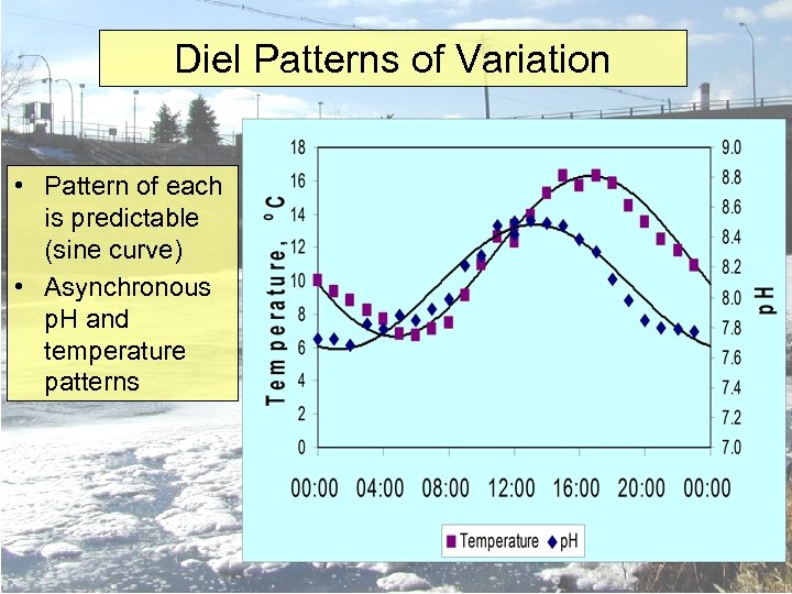Diel Patterns of Variation • Pattern of each is predictable (sine curve) • Asynchronous p. H and temperature patterns

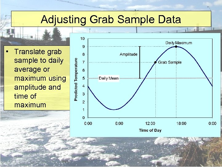Adjusting Grab Sample Data • Translate grab sample to daily average or maximum using amplitude and time of maximum

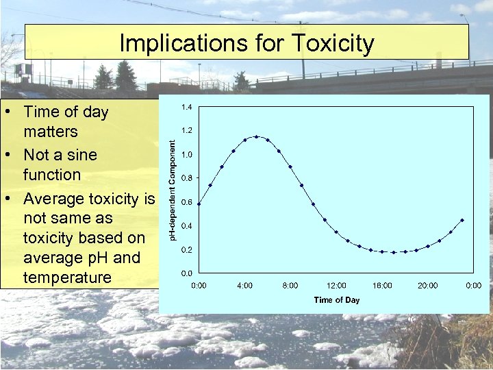Implications for Toxicity • Time of day matters • Not a sine function • Average toxicity is not same as toxicity based on average p. H and temperature

Empirical Seasonal Pattern • Driven by pattern observed in recent historical record • Temperature shows strong seasonal variation in mean; tracking air temperature • p. H shows strong seasonal variation in amplitude; result of biological activity

Seasonal Variation: Temperature • Strong pattern • Monthly time step • Importance of physical processes

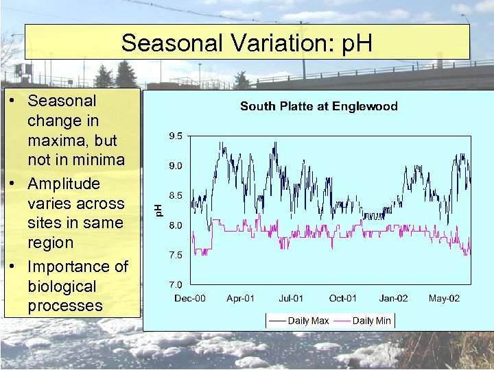Seasonal Variation: p. H • Seasonal change in maxima, but not in minima • Amplitude varies across sites in same region • Importance of biological processes

Next Task: Ammonia Trajectory • Initial concentration determined by mass balance calculations • Change in concentration d/s affected strongly by biological processes (i. e. , nonconservative behavior) • Dominant process: nitrification • Others: uptake (-), ammonification (+) • Model represents a net loss rate

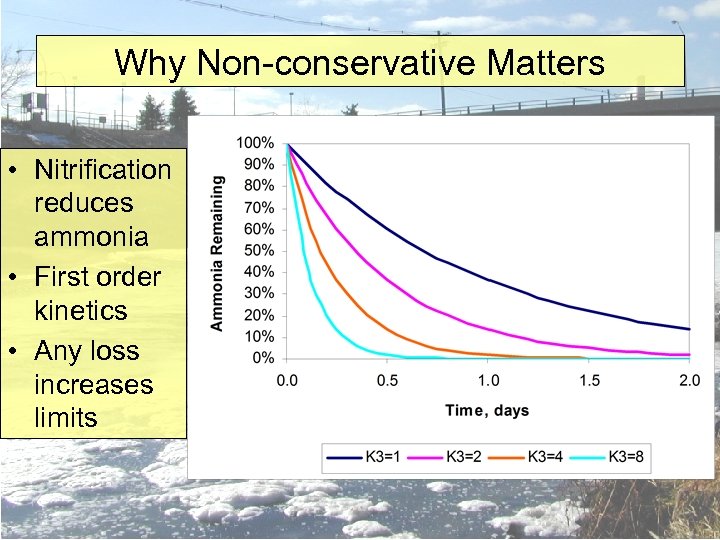Why Non-conservative Matters • Nitrification reduces ammonia • First order kinetics • Any loss increases limits

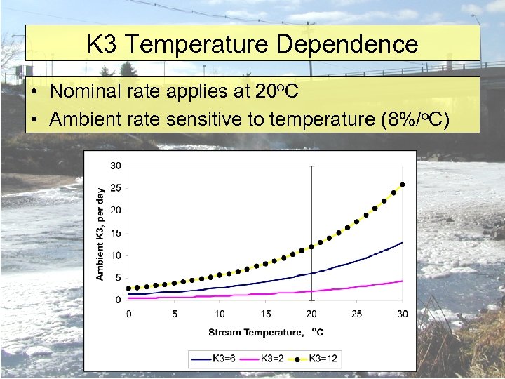K 3 Temperature Dependence • Nominal rate applies at 20 o. C • Ambient rate sensitive to temperature (8%/o. C)

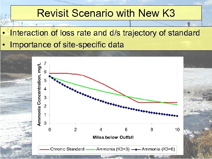Revisit Scenario with New K 3 • Interaction of loss rate and d/s trajectory of standard • Importance of site-specific data

Next Task: Linking Limits to Standards • AMMTOX sets monthly limits by manual iteration (i. e. , trial and error) • Aiming for maximum effluent concentration such that instream ammonia will not exceed standard at any point downstream

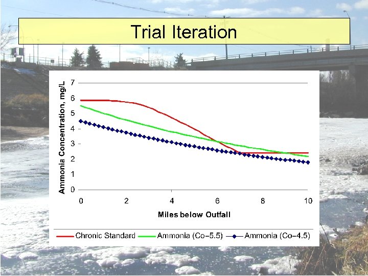Trial Iteration

Organization of AMMTOX • Recurrence model – Defines setpoint conditions, integral to mapping downstream trajectory of toxicity • Reach Model – Predicts downstream pattern of stream standard based on expected spatial patterns in p. H and temperature – Predicts downstream changes in total ammonia based on first order kinetics – Employs graphical approach for setting permit limits

Section 2: Data Needs and Sources • Setpoint Determination – Grab samples from equilibrium stream conditions; 3 -5 yrs, weekly-monthly – Diel patterns of variation for p. H and temperature (amplitude, time of max) • Default (3 levels for p. H) • User supplied (confirm or replace default) – Ecological Conditions • Implied by classification (warm vs. cold) • Local knowledge of fish community

Sampling Site Selection • Ideal site: far enough downstream for rebound to be complete, yet not influenced by tributaries, etc. • Practical site – Upstream OK if too many confounding influences downstream – Small effluent: upstream or 2 -4 mi downstream – Large effluent: trajectory based on interim sites

Site-Specific Characterization of Diel Patterns of Variation • Summer (July-August best) • Low flow • Data logger: 15 -min intervals; get amplitude and time of max • Grab: sunrise for minima, mid- to late afternoon for maxima; get amplitude • With either approach, a few sunny days will determine usefulness of defaults

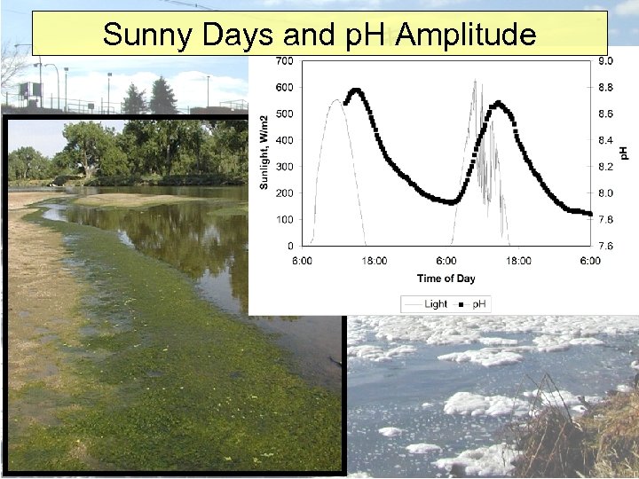Sunny Days and p. H Amplitude

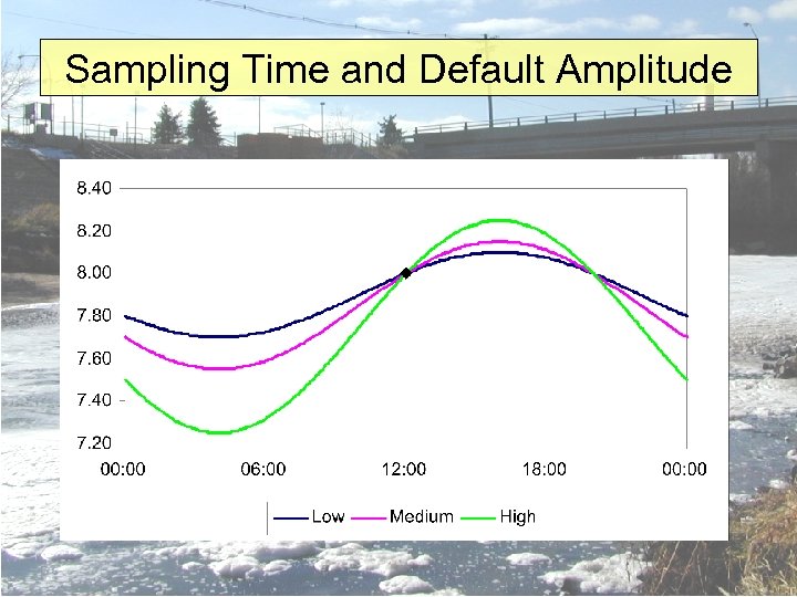Sampling Time and Default Amplitude

Define Ecological Setting for Reach Model • Are salmonids present? – Default assumption might be yes for Cold water classification – Affects p. H component (applies to acute and chronic standards) • Are Early Life Stages (ELS) present? – Must specify for each month – Applies to all species in fish community – Affects temperature component (does not apply to acute)

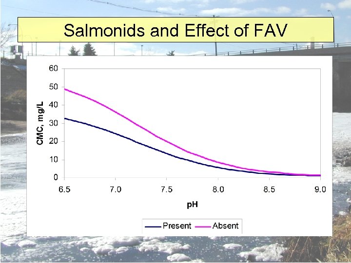Salmonids and Effect of FAV

Acute Values (CMC) • • 1 -h average Nonlinear function of p. H Not a function of temperature Linear function of FAV – Salmonids present: 11. 23 – Salmonids absent: 16. 8

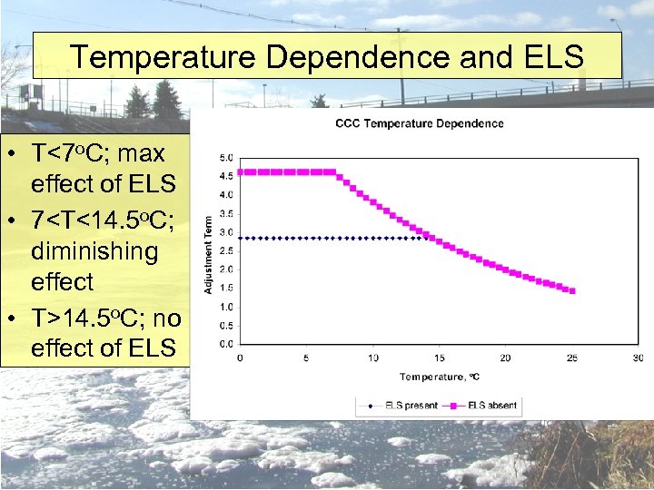Temperature Dependence and ELS • T<7 o. C; max effect of ELS • 714. 5 o. C; no effect of ELS

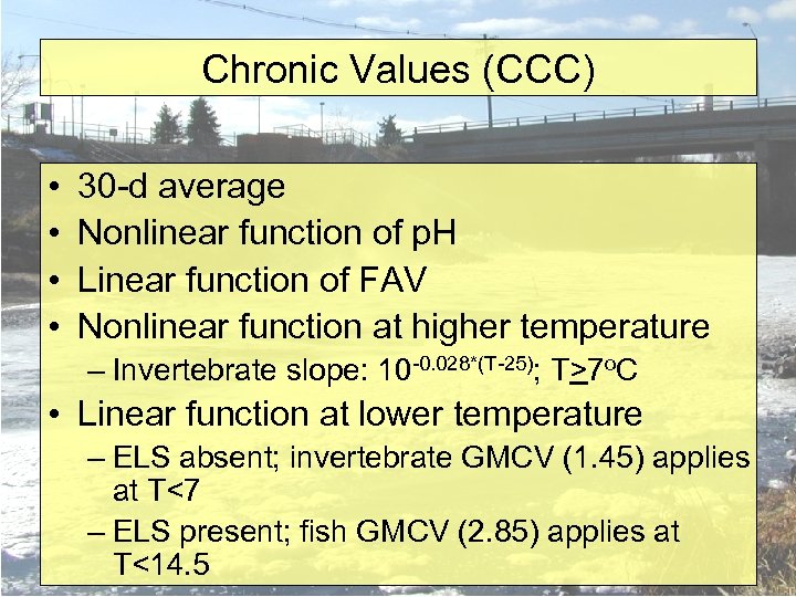Chronic Values (CCC) • • 30 -d average Nonlinear function of p. H Linear function of FAV Nonlinear function at higher temperature – Invertebrate slope: 10 -0. 028*(T-25); T>7 o. C • Linear function at lower temperature – ELS absent; invertebrate GMCV (1. 45) applies at T<7 – ELS present; fish GMCV (2. 85) applies at T<14. 5

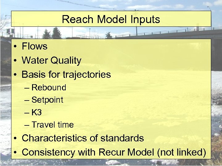Reach Model Inputs • Flows • Water Quality • Basis for trajectories – Rebound – Setpoint – K 3 – Travel time • Characteristics of standards • Consistency with Recur Model (not linked)

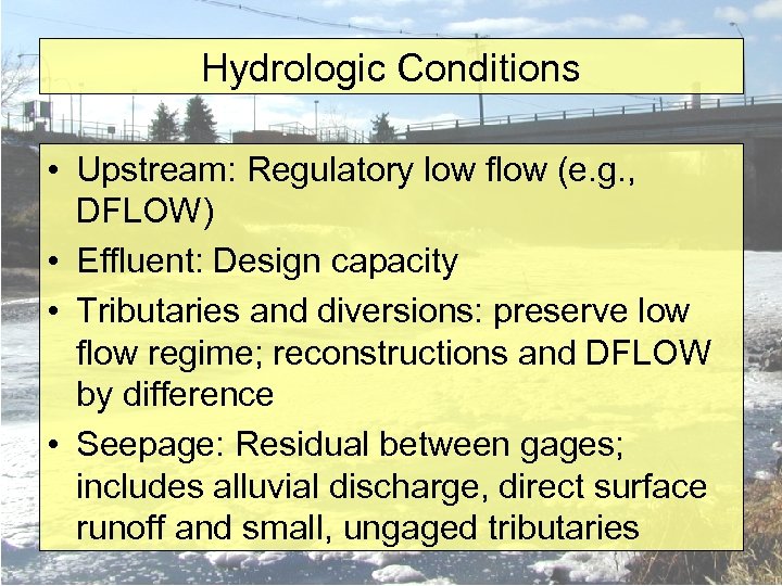Hydrologic Conditions • Upstream: Regulatory low flow (e. g. , DFLOW) • Effluent: Design capacity • Tributaries and diversions: preserve low flow regime; reconstructions and DFLOW by difference • Seepage: Residual between gages; includes alluvial discharge, direct surface runoff and small, ungaged tributaries

Input Water Quality • Avoid worst of worst scenarios • Upstream: average or median • Effluent (p. H, temperature): average or median • Seepage: average or median • Diversions: no direct effect on WQ

Rebound Rates • Default rates used in AMMTOX – p. H: 0. 2 units per mile – Temperature: 0. 7 o. C per mile • Site-specific rates are very rare • Produces gradual, linear shift toward setpoint conditions

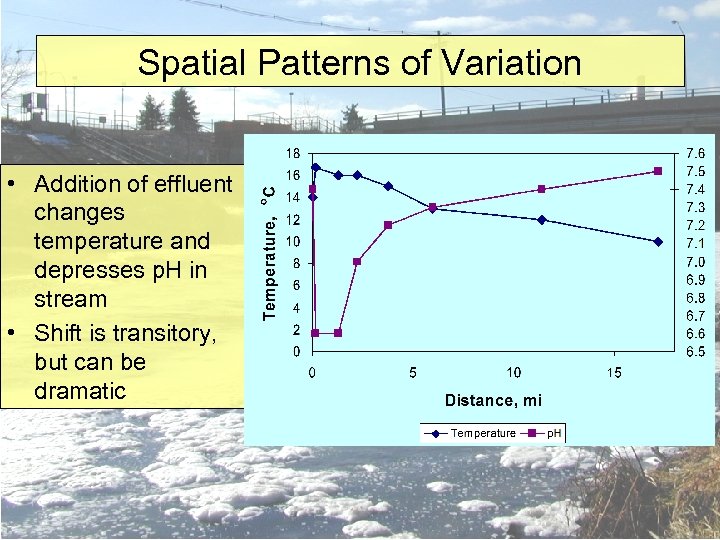Spatial Patterns of Variation • Addition of effluent changes temperature and depresses p. H in stream • Shift is transitory, but can be dramatic

Ammonia Loss Rate • Measured for many CO streams • Wide range of values; generous default • Study design considerations – Paired samples d/s of mixing zone – Travel time critical; must be able to see change in concentration – Detection limit and resolving power – Implications for DO modeling – Dilution by seepage vs. biological decay

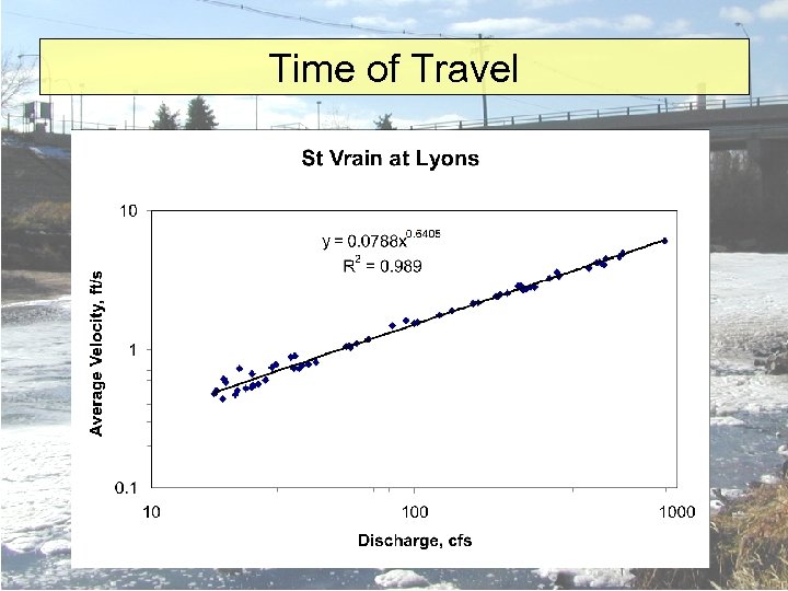
Velocity • Channel Geometry – Default – Site-specific: USGS Surface-water Measurements • Manning’s Eqn • Fixed Value; enter manually by reach • Special Considerations – Acute and chronic can be set separately – Multiple equations or approaches can be used when proper links are established

Time of Travel

Design of Basic Sampling Program • What – Stream: p. H, temperature, time, ammonia (u/s) – Effluent: p. H, temperature • When – Stream: biweekly or monthly – Effluent: individual, not DMR summary • Where – Upstream – Downstream (equilibrium conditions) • Supplemental – – Ammonia loss rate Diel variation in p. H and temperature Seepage Velocity