Algorithms Prof Dr Péter Iványi One of

Algorithms Prof. Dr. Péter Iványi

One of the oldest algorithms • bc. IV century, Alexandria, Euclides – Largest common denominator of two integers • Lets assume a and b positive integer number and the largest common denominator is ( a , b )

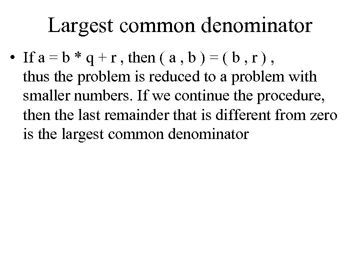Largest common denominator • If a = b * q + r , then ( a , b ) = ( b , r ) , thus the problem is reduced to a problem with smaller numbers. If we continue the procedure, then the last remainder that is different from zero is the largest common denominator

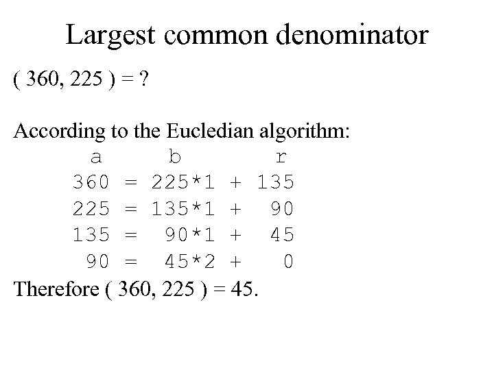Largest common denominator ( 360, 225 ) = ? According to the Eucledian algorithm: a b r 360 = 225*1 + 135 225 = 135*1 + 90 135 = 90*1 + 45 90 = 45*2 + 0 Therefore ( 360, 225 ) = 45.

Programming • Two basic concepts: – Description of relations between quantities and information x+y – Evaluation of these relations, where values are substituted into the expression x = 2 y = 3 2+3 = 5

Operations • We can specify simple operations on every data • For example: – Numbers: addition, subtraction, multiplication, . . . – Characters: Concatenate, sort, . . . • A programmer creates a program such simple operations

Information • Information is describd as data • There are different types of data: – Simple, (atomic, not divisible), like numbers – Complex, like number series • Although data represents the information, but the interpretation is up to us • For example 13. 51 can represent – temperature – time – distance

Programming, practical approach • To divide up the problem to simple operations (steps) that a computer can understand • The program: It is a sequence of operations that can be understood by a computer and that solves a problem.

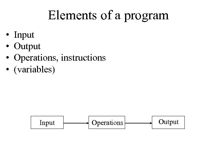Elements of a program • • Input Output Operations, instructions (variables) Input Operations Output

Input and output • Input – Keyboard – Mouse – File – Serial port, etc • Output – Screen – File – Serial port, etc

Variables • We store data in variables • Name – Denotes a storage place • Value – The stored data • Assigning – We put a data into a storage place

Data, simple • What kind of data can we store? • Numbers (bináris szám) – Integer – Real – Complex, etb • Characters – Binary number is converted to character • The same data can be stored in different ways – 1, ‘ 1’, “ 1”

Derived, complex data • • • Character series, string, Vectors Matrices Lists Etc. • Depends on the programming language!

Operations • Manipulating data • Arithmetic: – +, -, *, / • Relational: – >, <, =, <=, >= • Logical – NOT, AND, OR

Order of operations • a=6+12*5 • Evaluation order, • How to, in what order to execute the operations? – Generally from left to right – Precedence • Priority of operations – Brackets • a=(6+12)*5 • a=6+(12*5)

Program, summarised • Program, consists of several programs • Properties of algorithms: – Can be executed (consits of simple steps) – Every step is well defined – After a finite number of steps it stops – It is valid for a defined set of input – It produces the appropriate output – It solves a specific problem

Algorithms, design of programs

Programming methodology • Until 1960 monolithic programming • Properties: – One programmer – one program – There is no structure in the program

Programming methodology • The most important criteria of a good program – It has a visibly good structure – It is well documented – It can be „proven” that it does what it should

Modular programming • The basis of design: decomposition – The complicated problem is divided in pieces – We create a solution for the pieces – We assemble the pieces

Guidelines • Divide and conquer – Divide the problem to modules – Modules do not „get into” each other’s data – Modules operate independently • Easier to detec mistakes • Easier to overview the task • Easier to modify

Guidelines • Hiding data – Modules work only with their own data • Delaying decisions – Decision is only made when it is necessary – If there is not enough information, delay the decision • An early decision may have to be modified later • Once a decision has been made, declare it – Write it down, or record it – So later no contradictory decision is made

Modular programming • Top-Down decomposition – The task is divided into subtasks, which are also divided into further subtasks, until their size is small enough that they can be handler. • Bottom-Up composition – We use already existing building blocks – We do not know how they will connect together, which will connect to which other one – These building blocks must already exist

Modular programming • Advantages: – Subprograms can be easily overviewed – Easy to create them – Easy to test them – Several modules can be developed at the same time (parallel development) – Easy to correct mistakes – Modules can be standardised – It is possible to create module libraries – Reusable modules

Structured programming • Go To Statement Considered Harmful. – DOI: 10. 1145/214748. 315722 • Dijkstra: • Based on the Top-Down dekomposition – The original problem is divided into subproblems. This is an abstract program which works on an abstract computer. It can be proven that it works according to specification. – Refinement, which reduces the abstraction, e. g. a subproblem is described in more detail, which runs on another abstract machine. Still possible to prove that is satisfies the specification. – Further refinement, until we reach the level of a real computer, with its instructions.

Structured programming • Outcome: – The resulting is provably correct. • Problem: – The required amount of work is large. • Solution: – We miss certain steps, and therefore an approximately correct program is created, which can be checked by tests

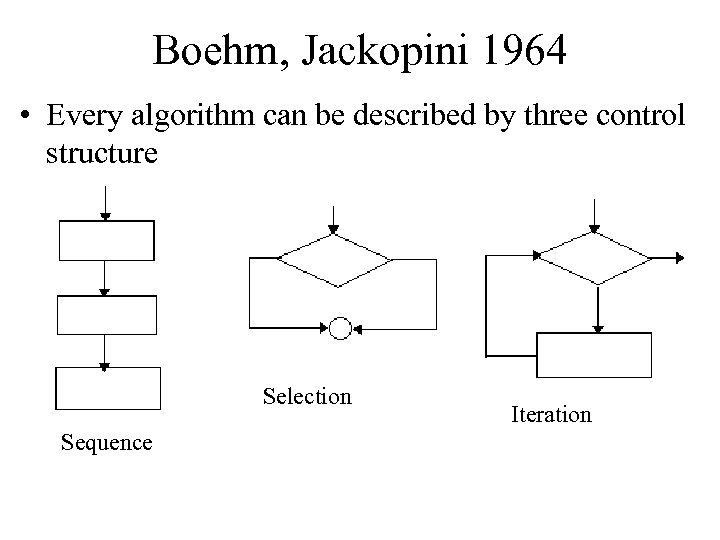Boehm, Jackopini 1964 • Every algorithm can be described by three control structure Selection Sequence Iteration

Mills 1968 • Proved theory of Boehm and Jackopini with certain conditions: – The basic structure of a program is a sequence – Every sequence has one entry and one exit point. An exit point of a module is an entry point of another module. – Every sequence can structured internally as required.

Graphic representation of algorithms • Pseudo code – Almost like sentences • Flowchart • Structogram – Nassi–Shneiderman diagram – Starting point is one rectangle, which can be divided. • . . .

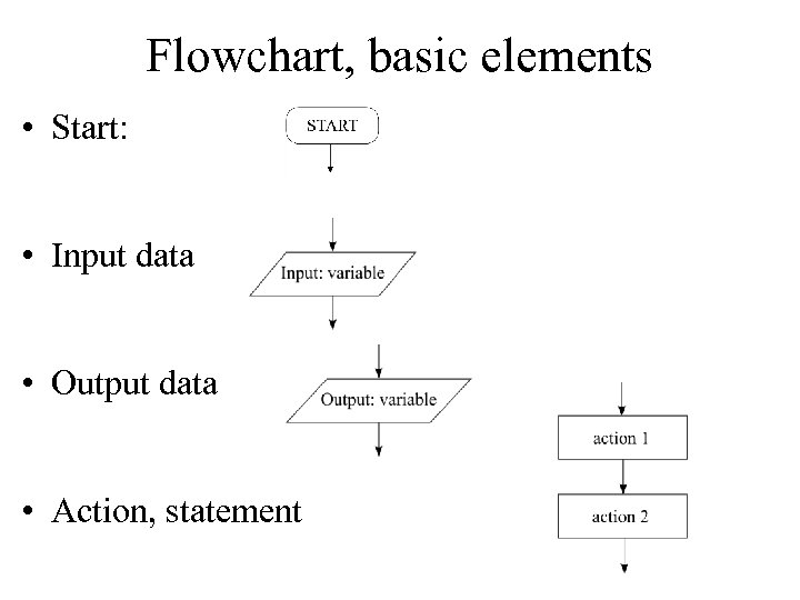Flowchart, basic elements • Start: • Input data • Output data • Action, statement

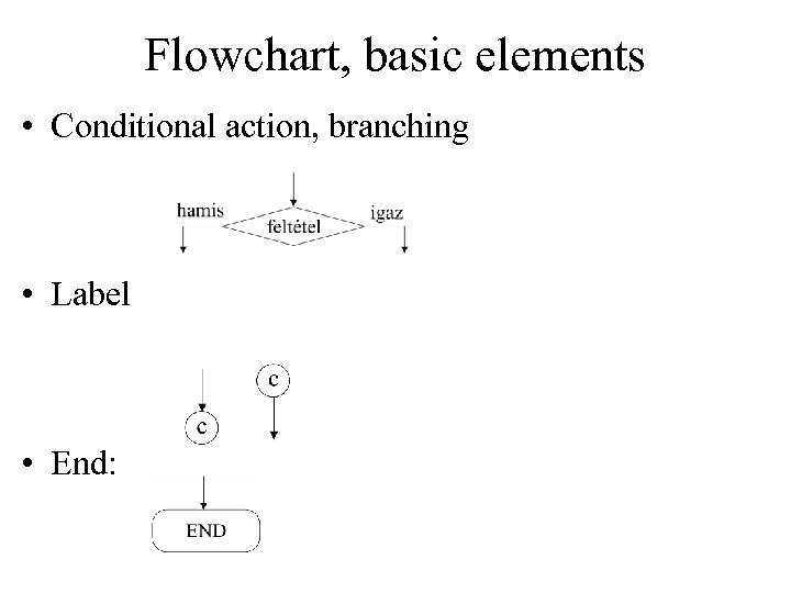Flowchart, basic elements • Conditional action, branching • Label • End:

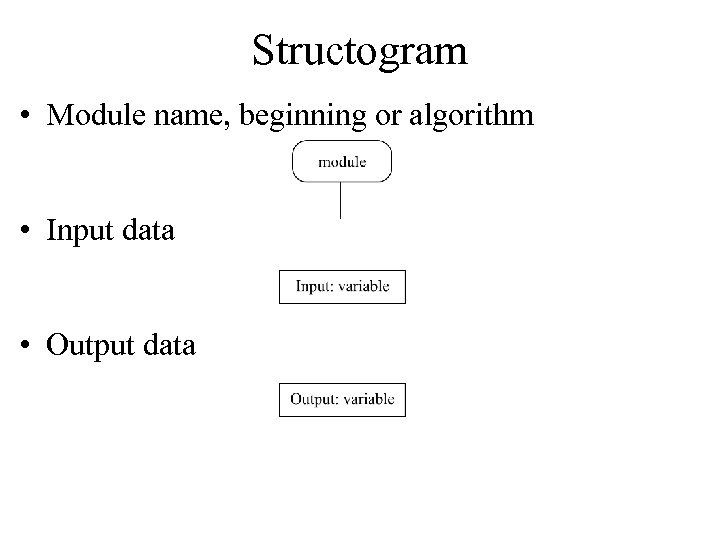Structogram • Module name, beginning or algorithm • Input data • Output data

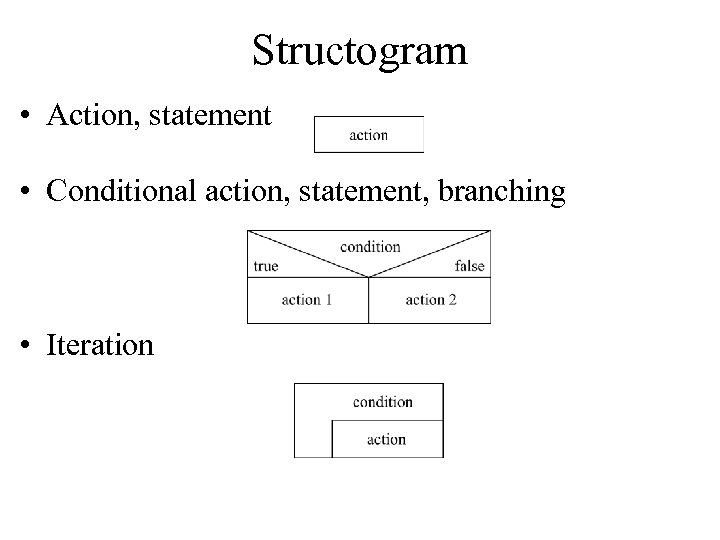Structogram • Action, statement • Conditional action, statement, branching • Iteration

Program execution • The computer executes one step after another one. • Control structure: deviation from the sequential order

Control structure • • Jump Conditional execution Multiple conditional execution Count controlled cycle, iteration, loop Pre-testing cycle, iteration, loop Post-testing cycle, iteration, loop (Subroutines)

Jump • The program continues at a new given point, not at the next step. • Usually results in structure that is difficult to understand • Not used in this semester!!!

Subprogram • Repeated task • Subtasks to separate • Names: – Subroutine – Procedure – Function

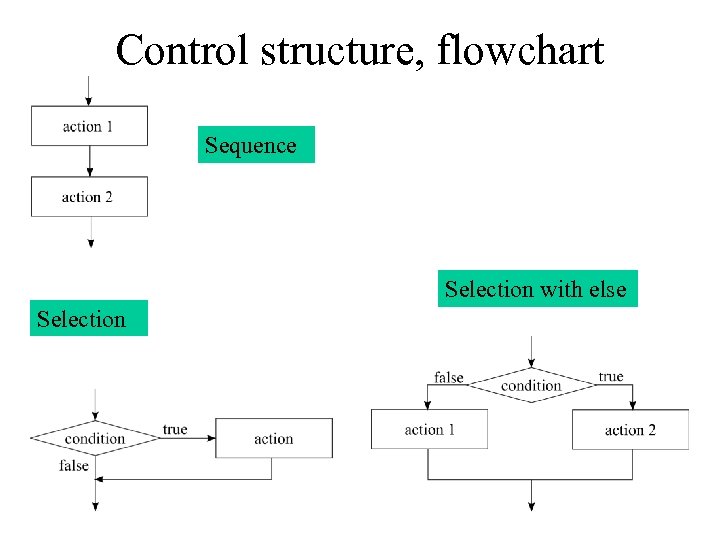Control structure, flowchart Sequence Selection with else Selection

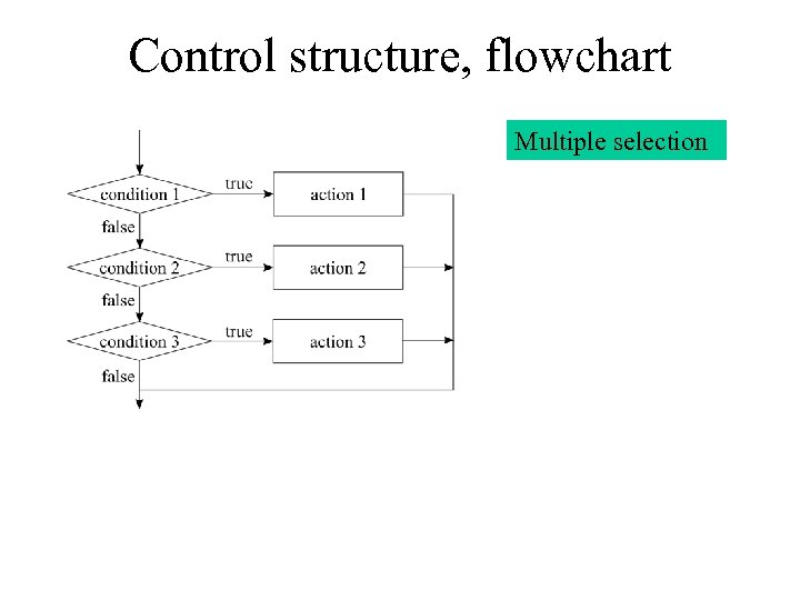Control structure, flowchart Multiple selection

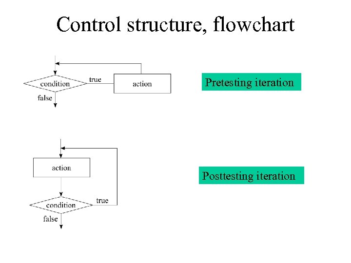Control structure, flowchart Pretesting iteration Posttesting iteration

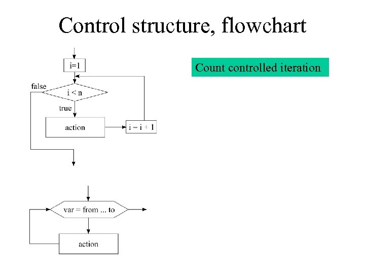Control structure, flowchart Count controlled iteration

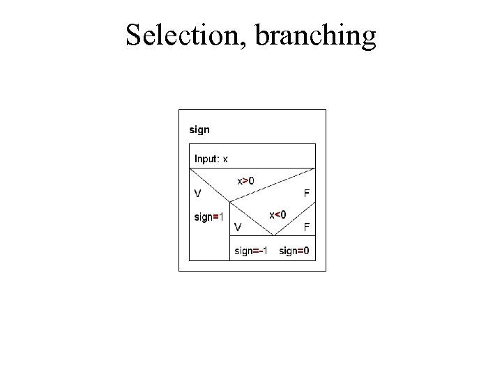
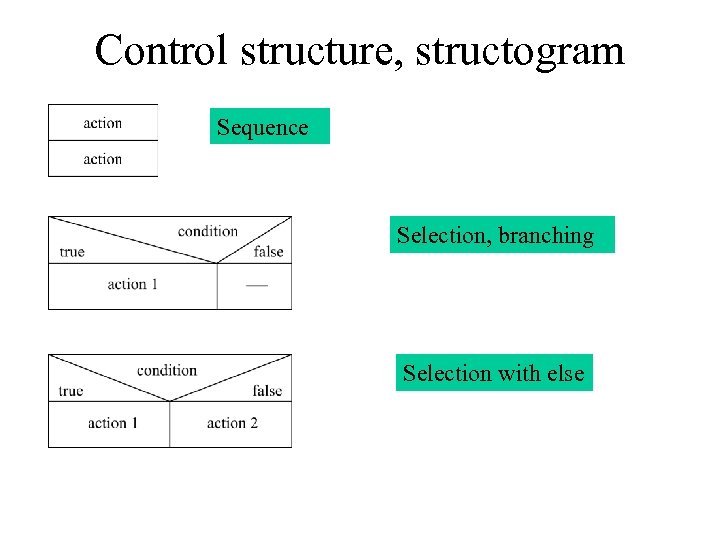Control structure, structogram Sequence Selection, branching Selection with else

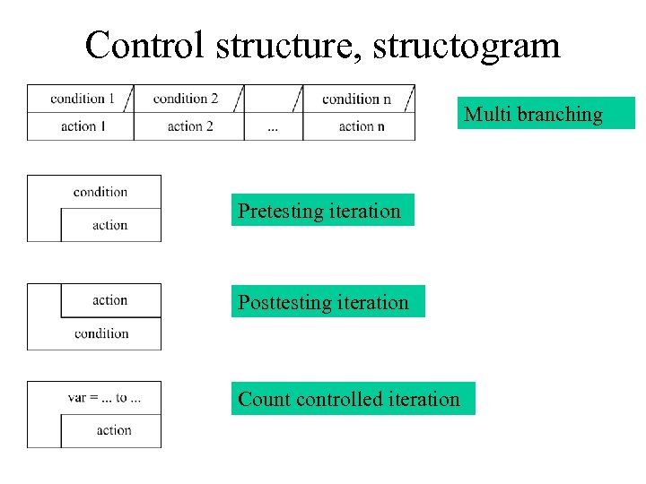Control structure, structogram Multi branching Pretesting iteration Posttesting iteration Count controlled iteration

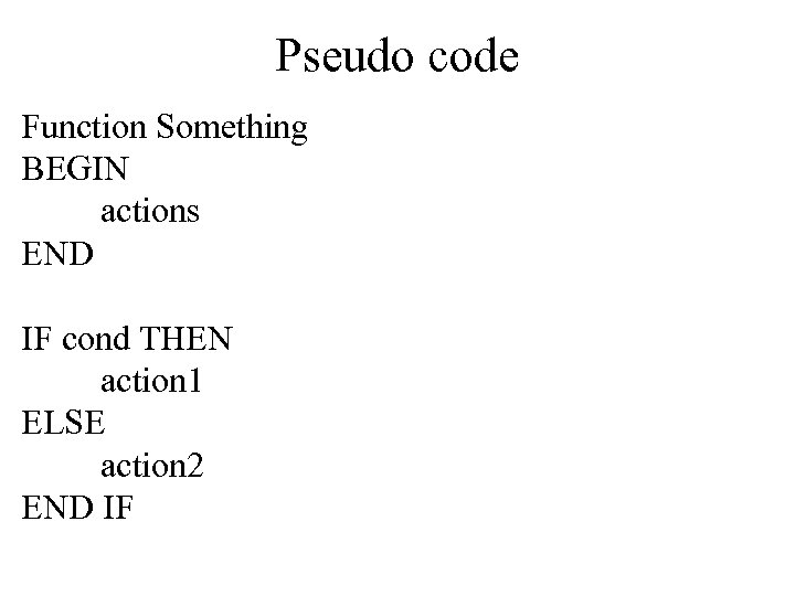Pseudo code Function Something BEGIN actions END IF cond THEN action 1 ELSE action 2 END IF

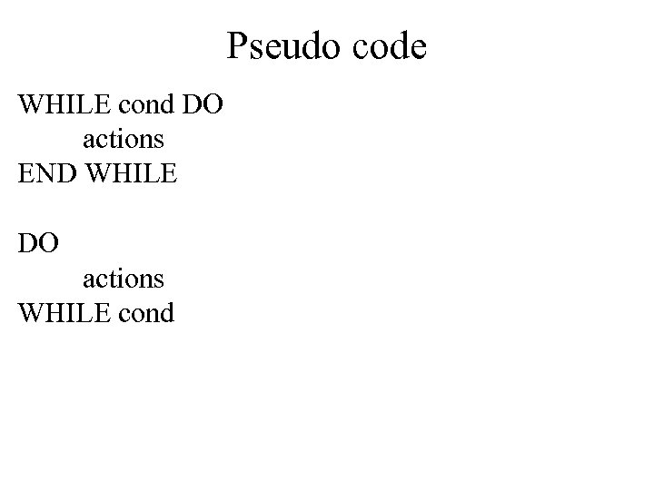Pseudo code WHILE cond DO actions END WHILE DO actions WHILE cond

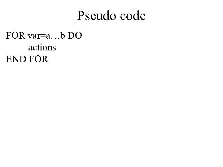Pseudo code FOR var=a…b DO actions END FOR

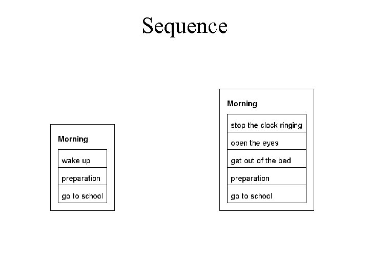Sequence

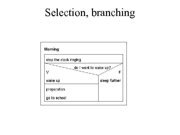Selection, branching

Selection, branching

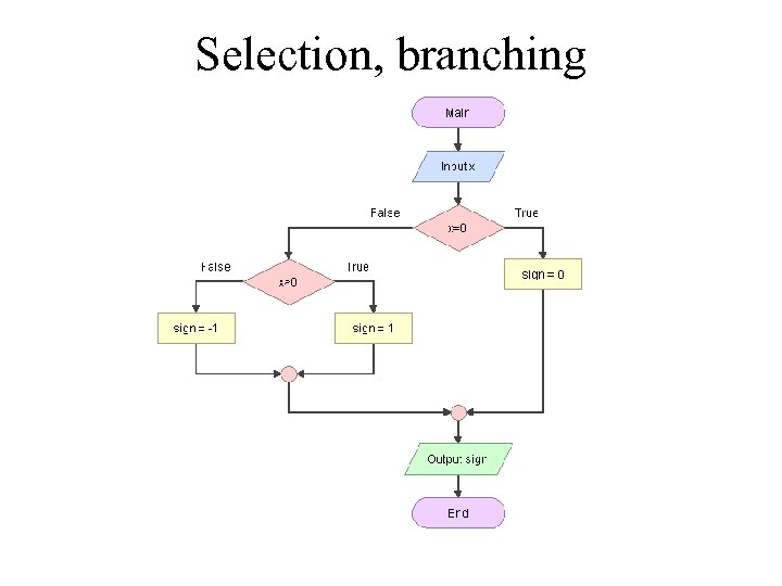Selection, branching

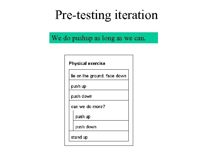Pre-testing iteration We do pushup as long as we can.

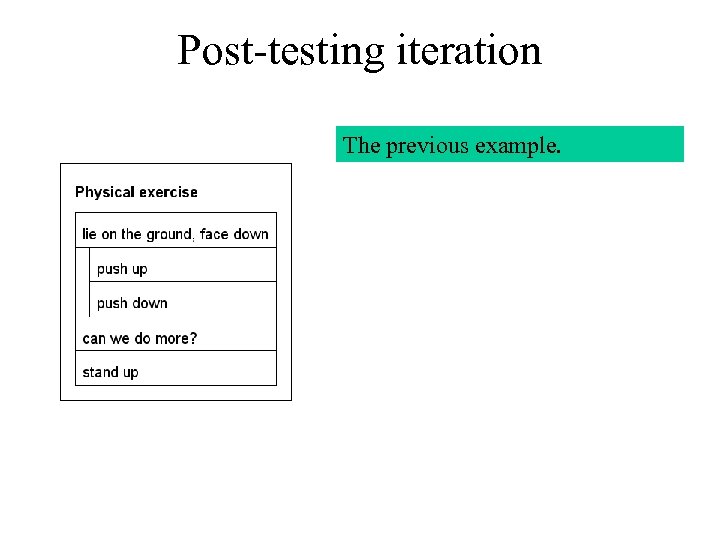Post-testing iteration The previous example.

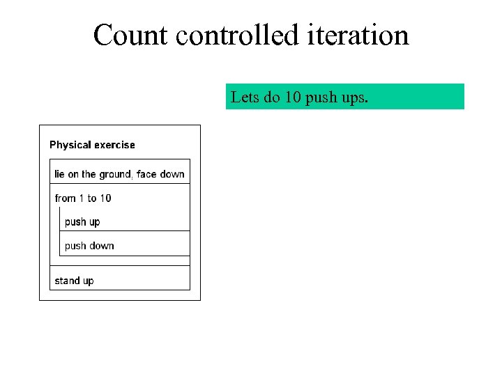Count controlled iteration Lets do 10 push ups.

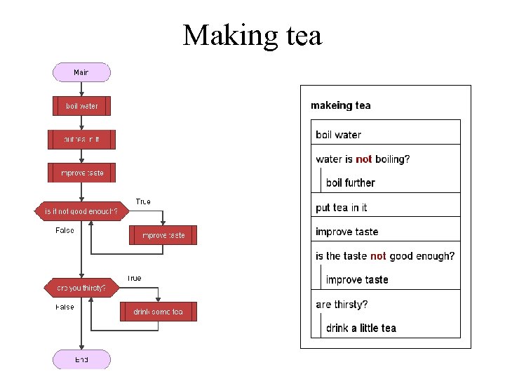Making tea

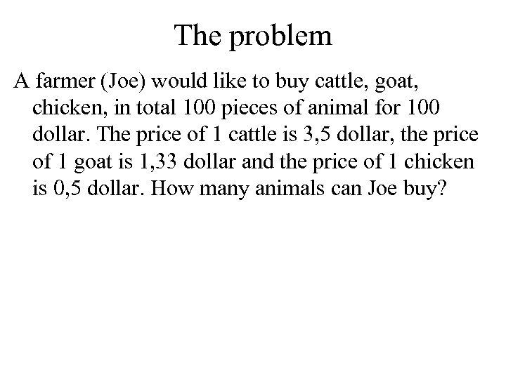The problem A farmer (Joe) would like to buy cattle, goat, chicken, in total 100 pieces of animal for 100 dollar. The price of 1 cattle is 3, 5 dollar, the price of 1 goat is 1, 33 dollar and the price of 1 chicken is 0, 5 dollar. How many animals can Joe buy?

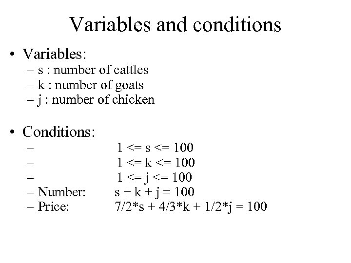Variables and conditions • Variables: – s : number of cattles – k : number of goats – j : number of chicken • Conditions: – 1 <= s <= 100 – 1 <= k <= 100 – 1 <= j <= 100 – Number: s + k + j = 100 – Price: 7/2*s + 4/3*k + 1/2*j = 100

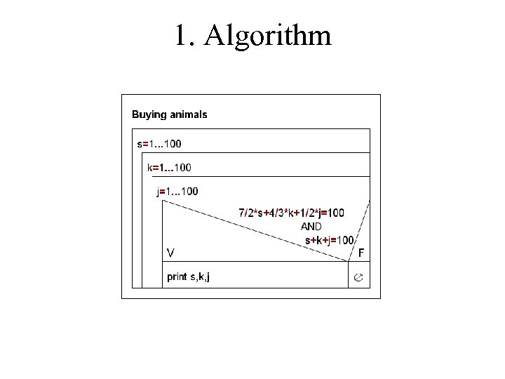1. Algorithm

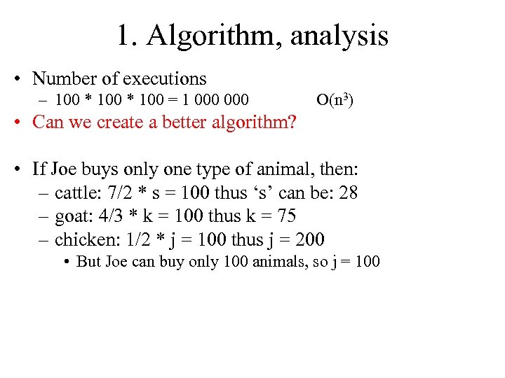1. Algorithm, analysis • Number of executions – 100 * 100 = 1 000 O(n 3) • Can we create a better algorithm? • If Joe buys only one type of animal, then: – cattle: 7/2 * s = 100 thus ‘s’ can be: 28 – goat: 4/3 * k = 100 thus k = 75 – chicken: 1/2 * j = 100 thus j = 200 • But Joe can buy only 100 animals, so j = 100

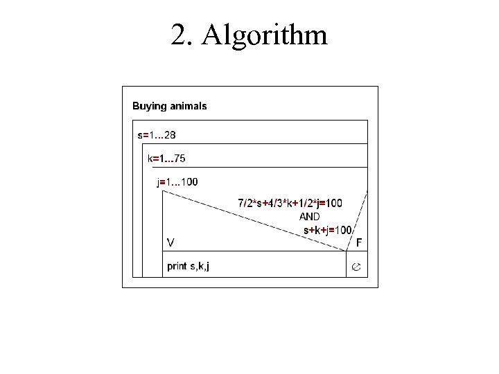2. Algorithm

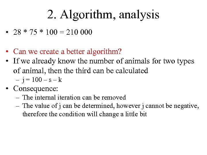2. Algorithm, analysis • 28 * 75 * 100 = 210 000 • Can we create a better algorithm? • If we already know the number of animals for two types of animal, then the third can be calculated – j = 100 – s – k • Consequence: – The internal iteration can be removed – The value of j can be determined, however j cannot be negative, therefore the condition will change a little bit

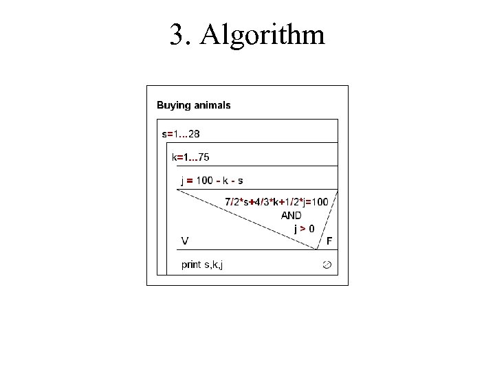3. Algorithm

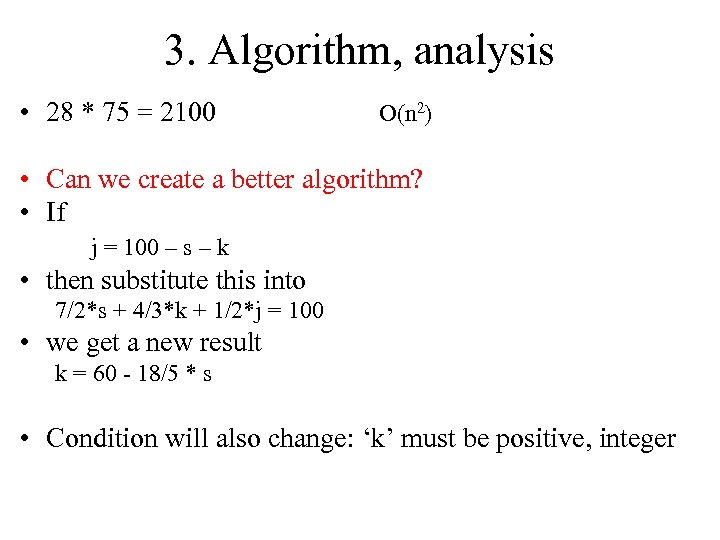3. Algorithm, analysis • 28 * 75 = 2100 O(n 2) • Can we create a better algorithm? • If j = 100 – s – k • then substitute this into 7/2*s + 4/3*k + 1/2*j = 100 • we get a new result k = 60 - 18/5 * s • Condition will also change: ‘k’ must be positive, integer

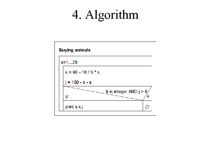4. Algorithm

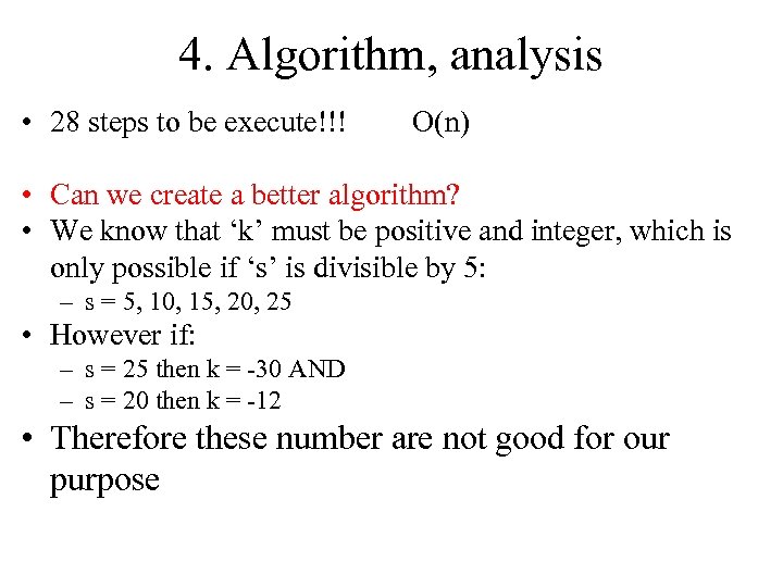4. Algorithm, analysis • 28 steps to be execute!!! O(n) • Can we create a better algorithm? • We know that ‘k’ must be positive and integer, which is only possible if ‘s’ is divisible by 5: – s = 5, 10, 15, 20, 25 • However if: – s = 25 then k = -30 AND – s = 20 then k = -12 • Therefore these number are not good for our purpose

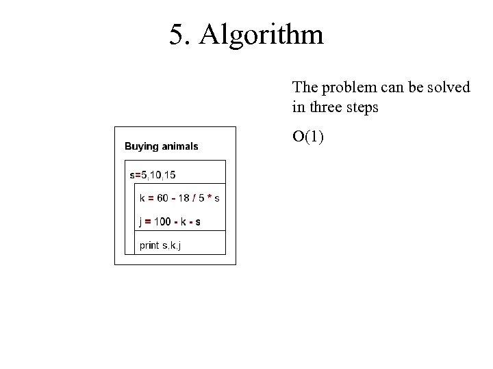5. Algorithm The problem can be solved in three steps O(1)

Programs • S T R U C T O R I Z E R: – http: //structorizer. fisch. lu/ • Flowgorithm: – http: //www. flowgorithm. org/index. htm