AICP Exam Review Planning Methods Blitz Bill Drummond

AICP Exam Review Planning Methods Blitz Bill Drummond City and Regional Planning Program Georgia Institute of Technology http: //drummond. gatech. edu/aicpexam. ppt

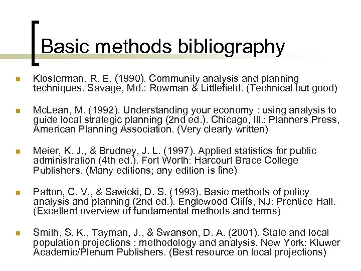
Basic methods bibliography n Klosterman, R. E. (1990). Community analysis and planning techniques. Savage, Md. : Rowman & Littlefield. (Technical but good) n Mc. Lean, M. (1992). Understanding your economy : using analysis to guide local strategic planning (2 nd ed. ). Chicago, Ill. : Planners Press, American Planning Association. (Very clearly written) n Meier, K. J. , & Brudney, J. L. (1997). Applied statistics for public administration (4 th ed. ). Fort Worth: Harcourt Brace College Publishers. (Many editions; any edition is fine) n Patton, C. V. , & Sawicki, D. S. (1993). Basic methods of policy analysis and planning (2 nd ed. ). Englewood Cliffs, NJ: Prentice Hall. (Excellent overview of fundamental methods and terms) n Smith, S. K. , Tayman, J. , & Swanson, D. A. (2001). State and local population projections : methodology and analysis. New York: Kluwer Academic/Plenum Publishers. (Best resource on local projections)

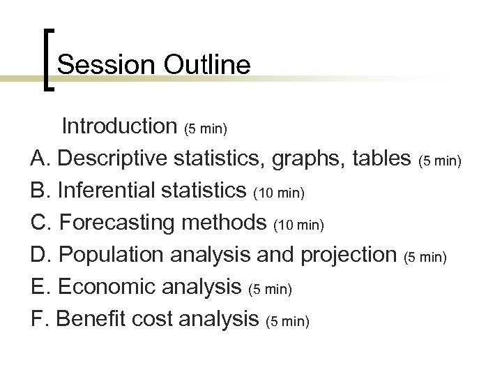
Session Outline Introduction (5 min) A. Descriptive statistics, graphs, tables (5 min) B. Inferential statistics (10 min) C. Forecasting methods (10 min) D. Population analysis and projection (5 min) E. Economic analysis (5 min) F. Benefit cost analysis (5 min)

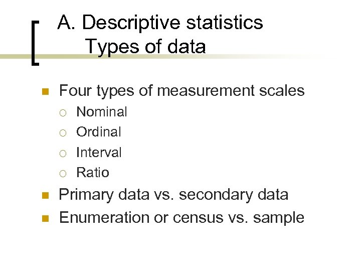
A. Descriptive statistics Types of data n Four types of measurement scales ¡ ¡ n n Nominal Ordinal Interval Ratio Primary data vs. secondary data Enumeration or census vs. sample

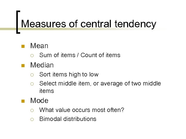
Measures of central tendency n Mean ¡ n Median ¡ ¡ n Sum of items / Count of items Sort items high to low Select middle item, or average of two middle items Mode ¡ ¡ What value occurs most often? Bimodal distributions

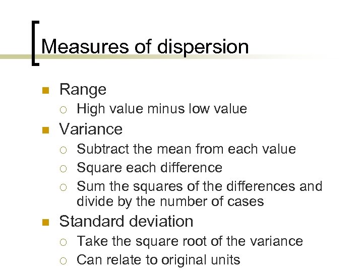
Measures of dispersion n Range ¡ n Variance ¡ ¡ ¡ n High value minus low value Subtract the mean from each value Square each difference Sum the squares of the differences and divide by the number of cases Standard deviation ¡ ¡ Take the square root of the variance Can relate to original units

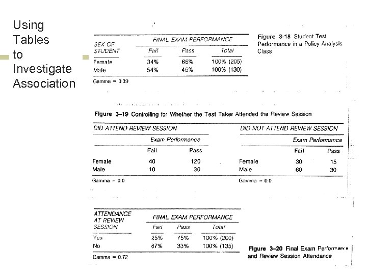
Using Tables to Investigate Association

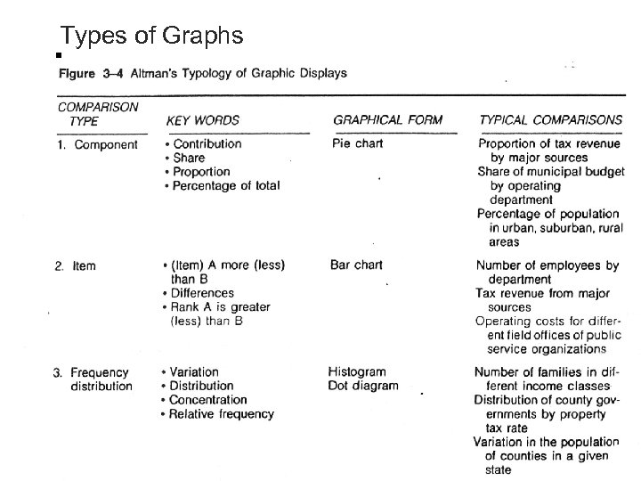
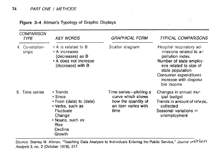
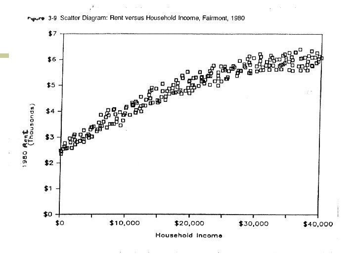
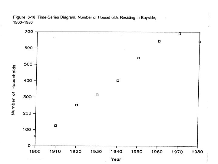
Types of Graphs

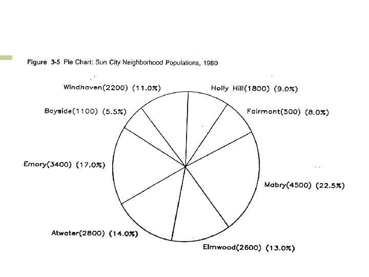
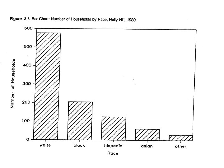
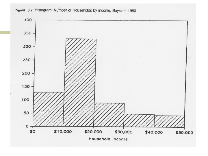
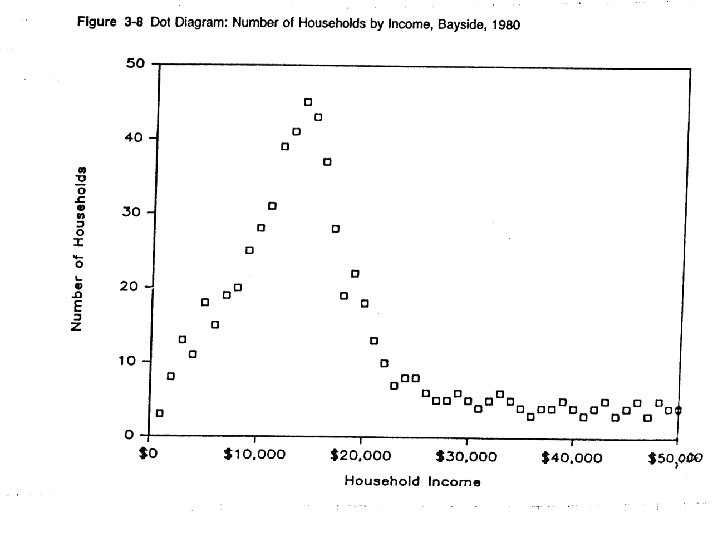
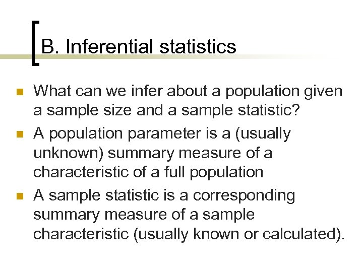
B. Inferential statistics n n n What can we infer about a population given a sample size and a sample statistic? A population parameter is a (usually unknown) summary measure of a characteristic of a full population A sample statistic is a corresponding summary measure of a sample characteristic (usually known or calculated).

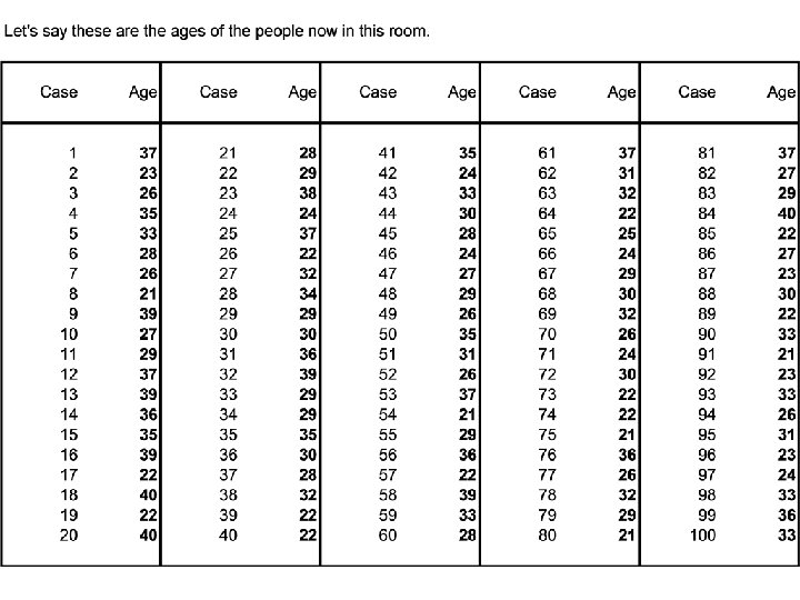
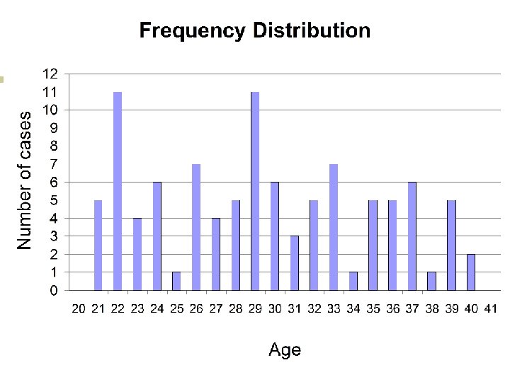
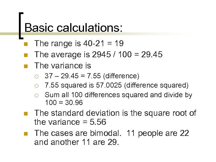
Basic calculations: n n n The range is 40 -21 = 19 The average is 2945 / 100 = 29. 45 The variance is ¡ ¡ ¡ n n 37 – 29. 45 = 7. 55 (difference) 7. 55 squared is 57. 0025 (difference squared) Sum all 100 differences squared and divide by 100 = 30. 96 The standard deviation is the square root of the variance = 5. 56 The cases are bimodal. 11 people are 22 and another 11 are 29.

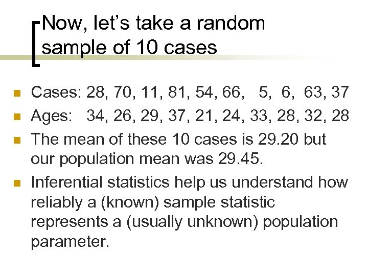
Now, let’s take a random sample of 10 cases n n Cases: 28, 70, 11, 81, 54, 66, 5, 6, 63, 37 Ages: 34, 26, 29, 37, 21, 24, 33, 28, 32, 28 The mean of these 10 cases is 29. 20 but our population mean was 29. 45. Inferential statistics help us understand how reliably a (known) sample statistic represents a (usually unknown) population parameter.

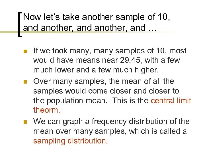
Now let’s take another sample of 10, and another, and … n n n If we took many, many samples of 10, most would have means near 29. 45, with a few much lower and a few much higher. Over many samples, the mean of all the samples would come closer and closer to the population mean. This is the central limit theorm. We can graph a frequency distribution of the mean over many samples, which is called a sampling distribution.

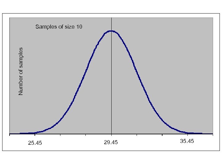
Number of samples Samples of size 10 25. 45 29. 45 35. 45

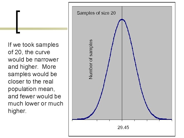
If we took samples of 20, the curve would be narrower and higher. More samples would be closer to the real population mean, and fewer would be much lower or much higher. Number of samples Samples of size 20 29. 45

Sample size and confidence limits n The standard error of the mean depends on the standard deviation of the population and the size of the sample. ¡ ¡ n n The smaller the SD of the population, the smaller the error. The larger the sample size, the smaller the error. Choosing an adequate sample size depends on the two factors listed above. You may want to be 90% certain that the mean of the sample will be within one year of the mean of the population.

Hypothesis testing n n A sample of 500 voters might show that 52% will vote for candidate X. That 52% could result from either ¡ ¡ n Random sampling fluctuation, or Over 50% of all voters will really vote for candidate X Hypothesis testing allows us to conclude with 95% certainty, that over 50% of voters support candidate X.

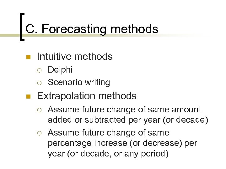
C. Forecasting methods n Intuitive methods ¡ ¡ n Delphi Scenario writing Extrapolation methods ¡ ¡ Assume future change of same amount added or subtracted per year (or decade) Assume future change of same percentage increase (or decrease) per year (or decade, or any period)

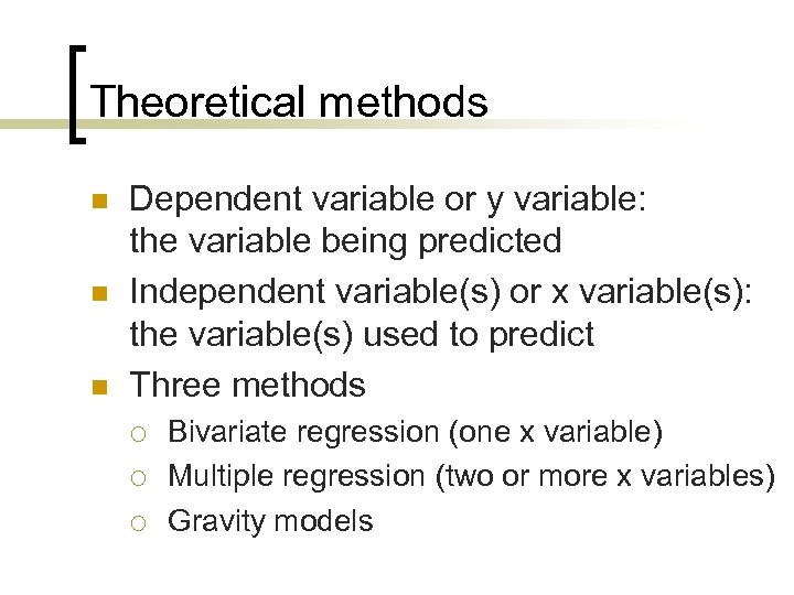
Theoretical methods n n n Dependent variable or y variable: the variable being predicted Independent variable(s) or x variable(s): the variable(s) used to predict Three methods ¡ ¡ ¡ Bivariate regression (one x variable) Multiple regression (two or more x variables) Gravity models

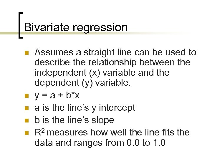
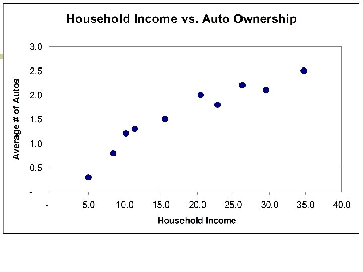
Bivariate regression n n Assumes a straight line can be used to describe the relationship between the independent (x) variable and the dependent (y) variable. y = a + b*x a is the line’s y intercept b is the line’s slope R 2 measures how well the line fits the data and ranges from 0. 0 to 1. 0

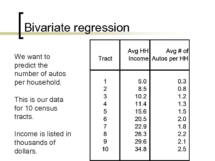
Bivariate regression We want to predict the number of autos per household. This is our data for 10 census tracts. Income is listed in thousands of dollars.

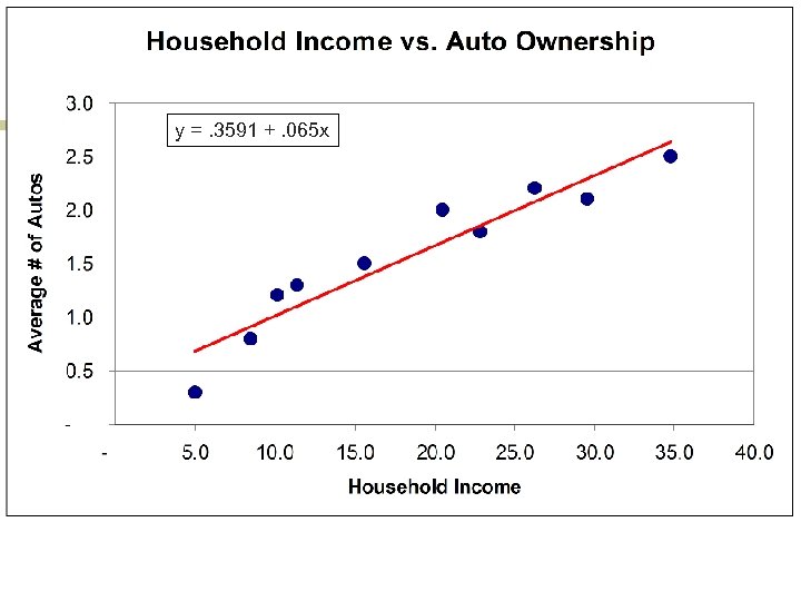
y =. 3591 +. 065 x

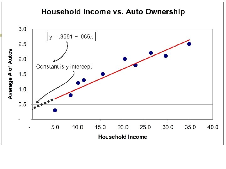
y =. 3591 +. 065 x Constant is y intercept

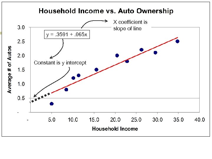
X coefficient is slope of line y =. 3591 +. 065 x Constant is y intercept

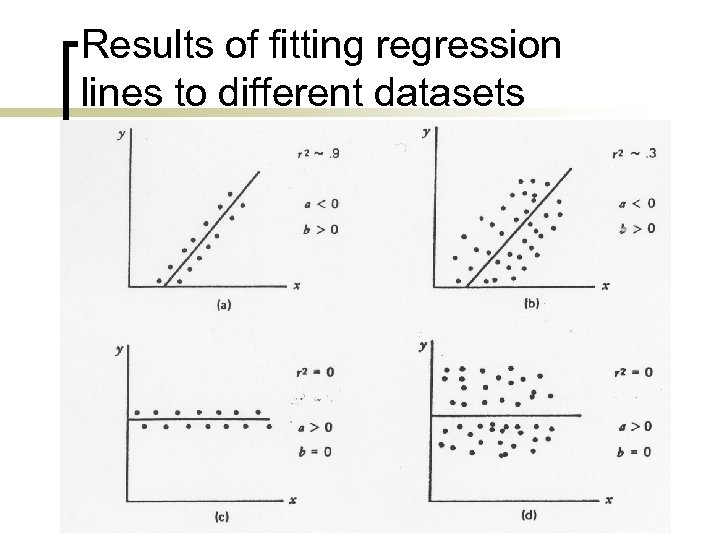
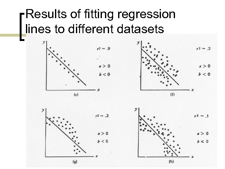
Results of fitting regression lines to different datasets

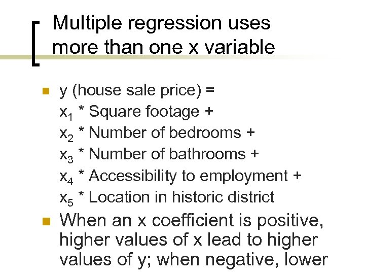
Multiple regression uses more than one x variable n y (house sale price) = x 1 * Square footage + x 2 * Number of bedrooms + x 3 * Number of bathrooms + x 4 * Accessibility to employment + x 5 * Location in historic district n When an x coefficient is positive, higher values of x lead to higher values of y; when negative, lower

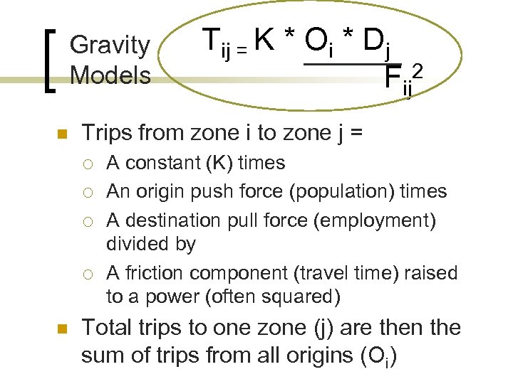
Gravity Models n Trips from zone i to zone j = ¡ ¡ n Tij = K * Oi * Dj Fij 2 A constant (K) times An origin push force (population) times A destination pull force (employment) divided by A friction component (travel time) raised to a power (often squared) Total trips to one zone (j) are then the sum of trips from all origins (Oi)

D. Population analysis and projection n An estimate is an indirect measure of a present or past condition that can not be directly measured. A projection (or prediction) is a conditional statement about the future. A forecast is a judgmental statement of what the analyst believes to be the most likely future.

Non-component projection methods n n Extrapolation with graphs Time series regression, with time (year) as the independent (x) variable Ratio methods comparing to similar areas Share methods using proportions of regional or state projections

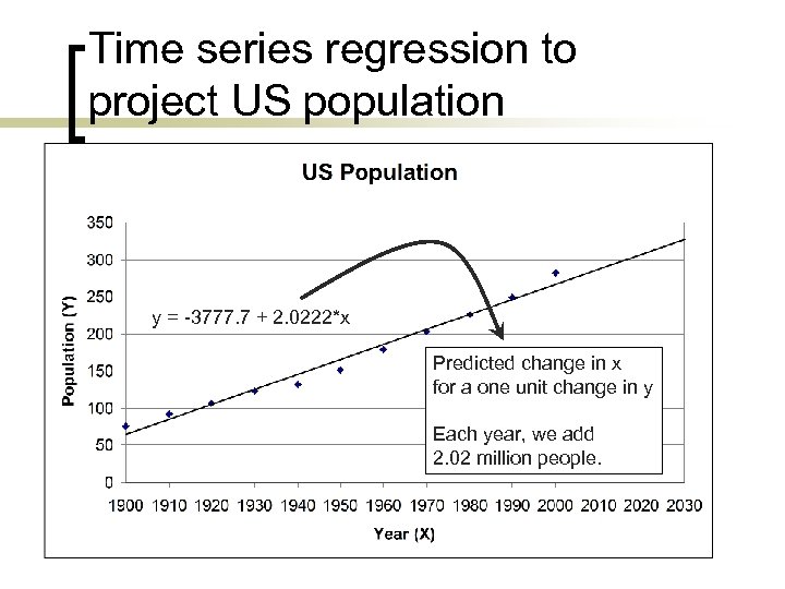
Time series regression to project US population y = -3777. 7 + 2. 0222*x Predicted change in x for a one unit change in y Each year, we add 2. 02 million people.

Cohort component models n n n We divide the population into cohorts by age (five years), sex, and race/ethnicity. Population change is subdivided into three components: births, deaths, migrants Calculate birth rates, survival rates, and migration rates for a recent period Extend those rates into the future, possibly adjusting them upward or downward Birth and death data is readily available; migration data is difficult, apart from Census years.

Migration notes n n n Migration can be projected as a function of changes in employment. Net migration = Inmigration - outmigration Net migration can estimated by the residual method: 1990 population: 100, 000 2000 population: 120, 000 1990 to 2000 births: 5, 000 1990 to 2000 deaths 3, 000 How many 1990 to 2000 inmigrants? (18, 000)

E: Economic analysis Economic base theory n Assumes two kinds of industry ¡ ¡ n Basic or export: sells to customers outside the area of analysis Service or non-basic: sells to customers within the area Economic base multiplier ¡ ¡ Total employment / basic employment A multiplier of 4. 0 says that 4 total jobs are created for every additional basic job

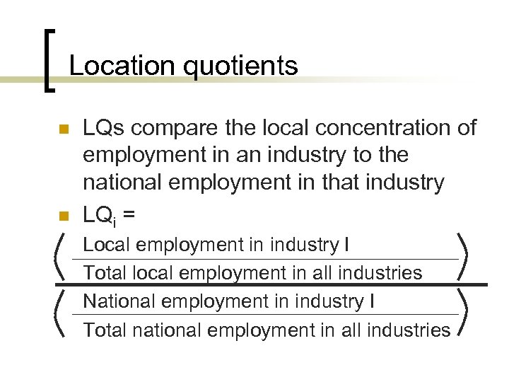
Location quotients n n LQs compare the local concentration of employment in an industry to the national employment in that industry LQi = Local employment in industry I Total local employment in all industries National employment in industry I Total national employment in all industries

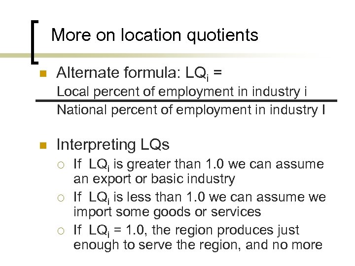
More on location quotients n Alternate formula: LQi = Local percent of employment in industry i National percent of employment in industry I n Interpreting LQs ¡ ¡ ¡ If LQi is greater than 1. 0 we can assume an export or basic industry If LQi is less than 1. 0 we can assume we import some goods or services If LQi = 1. 0, the region produces just enough to serve the region, and no more

Shift share analysis n Shift share analysis interprets changes in an industry’s local employment (over a period of x years) in terms of three components: ¡ ¡ ¡ National share: how much would local industry employment have changed if it mirrored changes in total national employment Industry mix: how much additional would it have changed if it mirrored national industry employment Local shift: how many additional jobs did the local industry gain or lose, presumably due to local competitive advantage or disadvantage.

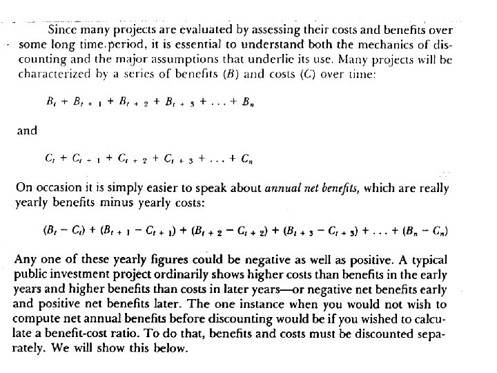
F. Project analysis and benefit cost analysis n n n Many public projects have high initial costs, then produce benefits for many years. $1, 000 of benefits in 10 years is less valuable than $1, 000 of benefits this year, because we could invest today’s $1, 000 and earn 10 years worth of interest. Discounting reduces benefits (and costs) in future years to account for the time value of money.

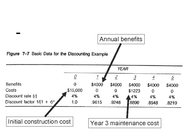
Annual benefits Initial construction cost Year 3 maintenance cost

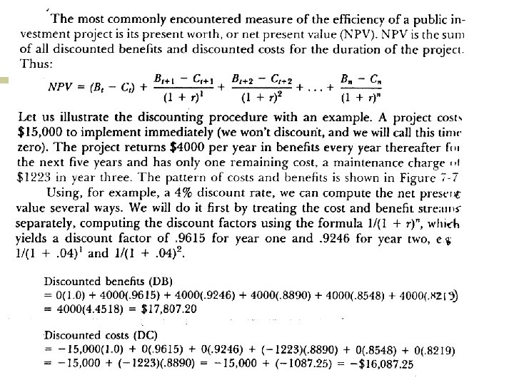
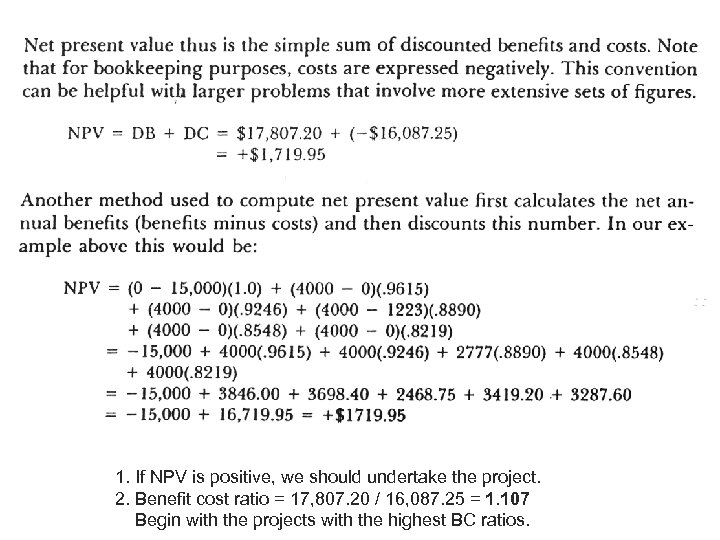
1. If NPV is positive, we should undertake the project. 2. Benefit cost ratio = 17, 807. 20 / 16, 087. 25 = 1. 107 Begin with the projects with the highest BC ratios.

AICP Exam Review Planning Methods Blitz Study hard, and Good luck on the exam! http: //drummond. gatech. edu/aicpexam. ppt